TEMPO L3 & L2
The Tropospheric Emissions: Monitoring of Pollution (TEMPO) products capture high-frequency air quality observations from a geostationary orbit over North America. Level-2 provides geolocated swath measurements at a few km resolution along the instrument’s scan, including trace gases such as NO₂, O₃, and HCHO, preserving the full spatial and temporal detail (hourly daytime coverage). Level-3 products aggregate these observations onto a regular latitude–longitude grid, reducing noise and filling gaps through spatial and temporal averaging (e.g., hourly or daily).
This notebook will use these two products:
TEMPO_NO2_L3 this is level 3 on a grid
TEMPO_O3TOT_L2 this is level 2 swath data
Note: In a virtual machine in AWS us-west-2, where NASA cloud data is, the point matchups are fast. In Colab, say, your compute is not in the same data region nor provider, and the same matchups might take 10x longer.
Prerequisites
The examples here use NASA EarthData and you need to have an account with EarthData. Make sure you can login.
# if needed
! pip install point - collocation cartopy
import earthaccess
earthaccess . login ()
TEMPO_NO2_L3
Create some points
Random global and only over land in 2024.
import pandas as pd
url = (
"https://raw.githubusercontent.com/"
"fish-pace/point-collocation/main/"
"examples/fixtures/points_1000_usa.csv"
)
df_points = pd . read_csv (
url ,
parse_dates = [ "time" ]
)
df = df_points [
( df_points [ "time" ] . dt . year == 2024 ) &
( df_points [ "land" ] == True )
]
print ( len ( df ))
df . head ()
lat
lon
time
land
5
42.919232
-107.118997
2024-02-07 19:04:58
True
22
32.033815
-87.504205
2024-03-12 19:18:24
True
106
44.862977
-110.808178
2024-05-21 15:46:24
True
127
36.649735
-80.935069
2024-04-24 22:48:36
True
138
29.592103
-95.889008
2024-03-30 03:06:23
True
Create the plan
%% time
import point_collocation as pc
short_name = "TEMPO_NO2_L3"
plan = pc . plan (
df ,
data_source = "earthaccess" ,
source_kwargs = {
"short_name" : short_name ,
"version" : "V03"
},
time_buffer = "1h"
)
plan . summary ( n = 2 )
Plan: 28 points → 30 unique granule(s)
  Points with 0 matches : 17
  Points with >1 matches: 10
  Time buffer: 0 days 01:00:00

First 2 point(s):
  [5] lat=42.9192, lon=-107.1190, time=2024-02-07 19:04:58: 3 match(es)
    → https://data.asdc.earthdata.nasa.gov/asdc-prod-protected/TEMPO/TEMPO_NO2_L3_V03/2024.02.07/TEMPO_NO2_L3_V03_20240207T172301Z_S007.nc
    → https://data.asdc.earthdata.nasa.gov/asdc-prod-protected/TEMPO/TEMPO_NO2_L3_V03/2024.02.07/TEMPO_NO2_L3_V03_20240207T182301Z_S008.nc
    → https://data.asdc.earthdata.nasa.gov/asdc-prod-protected/TEMPO/TEMPO_NO2_L3_V03/2024.02.07/TEMPO_NO2_L3_V03_20240207T192301Z_S009.nc
  [22] lat=32.0338, lon=-87.5042, time=2024-03-12 19:18:24: 2 match(es)
    → https://data.asdc.earthdata.nasa.gov/asdc-prod-protected/TEMPO/TEMPO_NO2_L3_V03/2024.03.12/TEMPO_NO2_L3_V03_20240312T174835Z_S009.nc
    → https://data.asdc.earthdata.nasa.gov/asdc-prod-protected/TEMPO/TEMPO_NO2_L3_V03/2024.03.12/TEMPO_NO2_L3_V03_20240312T184835Z_S010.nc
CPU times: user 1.55 s, sys: 214 ms, total: 1.76 s
Wall time: 16.2 s
Look at the variables
We will open a file with datatree and see what groups it has (if any). It does have groups; the latitude, longitude is at the base level: / and the product is in /product. We want vertical_column_troposphere which is the NO2. So we create a profile for TEMPO. We open a dataset with the profile to make sure it looks good.
%% time
tempo = {
'xarray_open' : 'dataset' ,
'merge' : [ '/' , '/product' ],
}
ds = plan . open_dataset ( 0 , open_method = tempo )
ds
open_method: {'xarray_open': 'dataset', 'merge': ['/', '/product'], 'open_kwargs': {'chunks': {}, 'engine': 'h5netcdf', 'decode_timedelta': False}, 'coords': 'auto', 'set_coords': True, 'dim_renames': None, 'auto_align_phony_dims': None, 'merge_kwargs': {}}
Geolocation auto detected with cf_xarray: ('longitude', 'latitude') — lon dims=('longitude',), lat dims=('latitude',); time dim='time' (1 step(s))
Points columns used: y='lat', x='lon', time='time'
CPU times: user 2.22 s, sys: 331 ms, total: 2.55 s
Wall time: 7.33 s
<xarray.Dataset> Size: 732MB
Dimensions:                                  (latitude: 2950, longitude: 7750,
                                              time: 1)
Coordinates:
  * latitude                                 (latitude) float32 12kB 14.01 .....
  * longitude                                (longitude) float32 31kB -168.0 ...
  * time                                     (time) datetime64[ns] 8B 2024-01...
Data variables:
    weight                                   (latitude, longitude) float32 91MB dask.array<chunksize=(590, 1550), meta=np.ndarray>
    vertical_column_troposphere              (time, latitude, longitude) float64 183MB dask.array<chunksize=(1, 738, 1938), meta=np.ndarray>
    vertical_column_troposphere_uncertainty  (time, latitude, longitude) float64 183MB dask.array<chunksize=(1, 738, 1938), meta=np.ndarray>
    vertical_column_stratosphere             (time, latitude, longitude) float64 183MB dask.array<chunksize=(1, 738, 1938), meta=np.ndarray>
    main_data_quality_flag                   (time, latitude, longitude) float32 91MB dask.array<chunksize=(1, 984, 2584), meta=np.ndarray>
Attributes: (12/40)
    history:                          2024-08-07T13:18:52Z: L2_regrid -v /tem...
    scan_num:                         1
    time_coverage_start:              2024-01-03T12:52:54Z
    time_coverage_end:                2024-01-03T13:32:40Z
    time_coverage_start_since_epoch:  1388321592.148252
    time_coverage_end_since_epoch:    1388323978.7368417
    ...                               ...
    title:                            TEMPO Level 3 nitrogen dioxide product
    collection_shortname:             TEMPO_NO2_L3
    collection_version:               1
    keywords:                         EARTH SCIENCE>ATMOSPHERE>AIR QUALITY>NI...
    summary:                          Nitrogen dioxide Level 3 files provide ...
coremetadata: \nGROUP = INVENTORYMET... Dimensions: latitude : 2950longitude : 7750time : 1
Coordinates: (3)
latitude
(latitude)
float32
14.01 14.03 14.05 ... 72.97 72.99
standard_name : latitude long_name : latitude comment : latitude at grid box center units : degrees_north valid_min : -90.0 valid_max : 90.0 array([14.01, 14.03, 14.05, ..., 72.95, 72.97, 72.99],
shape=(2950,), dtype=float32) longitude
(longitude)
float32
-168.0 -168.0 ... -13.03 -13.01
standard_name : longitude long_name : longitude comment : longitude at grid box center units : degrees_east valid_min : -180.0 valid_max : 180.0 array([-167.99, -167.97, -167.95, ..., -13.05, -13.03, -13.01],
shape=(7750,), dtype=float32) time
(time)
datetime64[ns]
2024-01-03T12:53:12.148251904
standard_name : time long_name : scan start time array(['2024-01-03T12:53:12.148251904'], dtype='datetime64[ns]') Data variables: (5)
weight
(latitude, longitude)
float32
dask.array<chunksize=(590, 1550), meta=np.ndarray>
long_name : sum of area weights comment : sum of Level 2 pixel overlap areas units : km^2
Array
Chunk
Bytes
87.21 MiB
3.49 MiB
Shape
(2950, 7750)
(590, 1550)
Dask graph
25 chunks in 2 graph layers
Data type
float32 numpy.ndarray
7750
2950
vertical_column_troposphere
(time, latitude, longitude)
float64
dask.array<chunksize=(1, 738, 1938), meta=np.ndarray>
long_name : troposphere nitrogen dioxide vertical column units : molecules/cm^2
Array
Chunk
Bytes
174.43 MiB
10.91 MiB
Shape
(1, 2950, 7750)
(1, 738, 1938)
Dask graph
16 chunks in 2 graph layers
Data type
float64 numpy.ndarray
7750
2950
1
vertical_column_troposphere_uncertainty
(time, latitude, longitude)
float64
dask.array<chunksize=(1, 738, 1938), meta=np.ndarray>
long_name : troposphere nitrogen dioxide vertical column uncertainty units : molecules/cm^2
Array
Chunk
Bytes
174.43 MiB
10.91 MiB
Shape
(1, 2950, 7750)
(1, 738, 1938)
Dask graph
16 chunks in 2 graph layers
Data type
float64 numpy.ndarray
7750
2950
1
vertical_column_stratosphere
(time, latitude, longitude)
float64
dask.array<chunksize=(1, 738, 1938), meta=np.ndarray>
long_name : stratosphere nitrogen dioxide vertical column units : molecules/cm^2
Array
Chunk
Bytes
174.43 MiB
10.91 MiB
Shape
(1, 2950, 7750)
(1, 738, 1938)
Dask graph
16 chunks in 2 graph layers
Data type
float64 numpy.ndarray
7750
2950
1
main_data_quality_flag
(time, latitude, longitude)
float32
dask.array<chunksize=(1, 984, 2584), meta=np.ndarray>
long_name : main data quality flag valid_min : 0 valid_max : 2 flag_meanings : normal suspicious bad flag_values : [0 1 2]
Array
Chunk
Bytes
87.21 MiB
9.70 MiB
Shape
(1, 2950, 7750)
(1, 984, 2584)
Dask graph
9 chunks in 2 graph layers
Data type
float32 numpy.ndarray
7750
2950
1
Attributes: (40)
history : 2024-08-07T13:18:52Z: L2_regrid -v /tempo/nas0/sdpc/liveroot/temposdpc/ops4/etc/l3.cfg
scan_num : 1 time_coverage_start : 2024-01-03T12:52:54Z time_coverage_end : 2024-01-03T13:32:40Z time_coverage_start_since_epoch : 1388321592.148252 time_coverage_end_since_epoch : 1388323978.7368417 product_type : NO2 processing_level : 3 processing_version : 3 sdpc_version : TEMPO_SDPC_v4.4.2 production_date_time : 2024-08-07T13:18:53Z begin_date : 2024-01-03 begin_time : 12:52:54 end_date : 2024-01-03 end_time : 13:32:40 local_granule_id : TEMPO_NO2_L3_V03_20240103T125254Z_S001.nc version_id : 3 pge_version : 1.0.0 shortname : TEMPO_NO2_L3 input_files : ['TEMPO_NO2_L2_V03_20240103T125254Z_S001G01.nc', 'TEMPO_NO2_L2_V03_20240103T125934Z_S001G02.nc', 'TEMPO_NO2_L2_V03_20240103T130611Z_S001G03.nc', 'TEMPO_NO2_L2_V03_20240103T131249Z_S001G04.nc', 'TEMPO_NO2_L2_V03_20240103T131926Z_S001G05.nc', 'TEMPO_NO2_L2_V03_20240103T132603Z_S001G06.nc'] geospatial_bounds : POLYGON((57.6000 -110.5000,53.5600 -108.3200,49.2200 -106.5200,44.3200 -104.9600,39.6000 -103.8000,33.9600 -102.7400,28.7400 -102.0000,22.8400 -101.3800,17.2600 -100.9600,17.2200 -85.2400,17.4800 -65.1200,21.9400 -64.1200,25.7600 -63.0400,29.6200 -61.7000,32.7800 -60.3800,36.3000 -58.6200,39.4000 -56.7600,42.1800 -54.7800,44.8400 -52.5400,47.7200 -49.6200,50.4000 -46.2800,52.7400 -42.6800,54.7200 -38.9200,56.3800 -35.0200,57.9600 -30.3200,59.1600 -25.6600,60.2400 -20.1000,61.2200 -20.0800,61.2000 -20.2600,61.4800 -20.2800,61.4400 -20.5400,62.8000 -20.5600,62.7200 -21.1000,63.5600 -21.1200,63.4600 -21.8400,63.7200 -21.9600,63.5600 -22.9800,63.4800 -24.4400,62.6600 -30.0600,61.5200 -38.4200,60.7600 -44.1800,59.9600 -51.1600,58.7800 -63.3000,58.2200 -71.1800,57.7800 -80.4600,57.6000 -90.7600,57.7600 -101.2800,58.2000 -110.5000,57.6000 -110.5000)) geospatial_bounds_crs : EPSG:4326 geospatial_lon_min : -110.5 geospatial_lon_max : -20.080002 geospatial_lat_min : 17.22 geospatial_lat_max : 63.719997 time_reference : 1980-01-06T00:00:00Z day_of_year : 3 project : TEMPO platform : Intelsat 40e source : UV-VIS hyperspectral imaging institution : Smithsonian Astrophysical Observatory creator_url : http://tempo.si.edu Conventions : CF-1.6, ACDD-1.3 title : TEMPO Level 3 nitrogen dioxide product collection_shortname : TEMPO_NO2_L3 collection_version : 1 keywords : EARTH SCIENCE>ATMOSPHERE>AIR QUALITY>NITROGEN OXIDES, EARTH SCIENCE>ATMOSPHERE>ATMOSPHERIC CHEMISTRY>NITROGEN COMPOUNDS>NITROGEN DIOXIDE summary : Nitrogen dioxide Level 3 files provide trace gas information on a regular grid covering the TEMPO field of regard for nominal TEMPO observations. Level 3 files are derived by combining information from all Level 2 files constituting a TEMPO East-West scan cycle. The files are provided in netCDF4 format, and contain information on tropospheric, stratospheric and total nitrogen dioxide vertical columns, ancillary data used in air mass factor and stratospheric/tropospheric separation calculations, and retrieval quality flags. The re-gridding algorithm uses an area-weighted approach. coremetadata :
GROUP = INVENTORYMETADATA
GROUPTYPE = MASTERGROUP
GROUP = ECSDATAGRANULE
OBJECT = LOCALGRANULEID
NUM_VAL = 1
VALUE = "TEMPO_NO2_L3_V03_20240103T125254Z_S001.nc"
END_OBJECT = LOCALGRANULEID
OBJECT = LOCALVERSIONID
NUM_VAL = 1
VALUE = ("RFC1321 MD5 = not yet calculated")
END_OBJECT = LOCALVERSIONID
OBJECT = PRODUCTIONDATETIME
NUM_VAL = 1
VALUE = "2024-08-07T13:18:53Z"
END_OBJECT = PRODUCTIONDATETIME
END_GROUP = ECSDATAGRANULE
GROUP = COLLECTIONDESCRIPTIONCLASS
OBJECT = SHORTNAME
NUM_VAL = 1
VALUE = "TEMPO_NO2_L3"
END_OBJECT = SHORTNAME
OBJECT = VERSIONID
NUM_VAL = 1
VALUE = 3
END_OBJECT = VERSIONID
END_GROUP = COLLECTIONDESCRIPTIONCLASS
GROUP = INPUTGRANULE
OBJECT = INPUTPOINTER
NUM_VAL = 6
VALUE = ("TEMPO_NO2_L2_V03_20240103T125254Z_S001G01.nc", "TEMPO_NO2_L2_V03_20240103T125934Z_S001G02.nc", "TEMPO_NO2_L2_V03_20240103T130611Z_S001G03.nc", "TEMPO_NO2_L2_V03_20240103T131249Z_S001G04.nc", "TEMPO_NO2_L2_V03_20240103T131926Z_S001G05.nc", "TEMPO_NO2_L2_V03_20240103T132603Z_S001G06.nc")
END_OBJECT = INPUTPOINTER
END_GROUP = INPUTGRANULE
GROUP = SPATIALDOMAINCONTAINER
GROUP = HORIZONTALSPATIALDOMAINCONTAINER
GROUP = GPOLYGON
OBJECT = GPOLYGONCONTAINER
CLASS = "1"
GROUP = GRINGPOINT
CLASS = "1"
OBJECT = GRINGPOINTLONGITUDE
NUM_VAL = 49
CLASS = "1"
VALUE = (-110.5, -108.32, -106.52, -104.96, -103.8, -102.74, -102, -101.38, -100.96, -85.24001, -65.12, -64.12, -63.04, -61.7, -60.38, -58.62, -56.76, -54.78, -52.54, -49.62, -46.28001, -42.68, -38.92, -35.02, -30.32001, -25.66, -20.10001, -20.08, -20.26001, -20.28, -20.54001, -20.56, -21.10001, -21.12001, -21.84, -21.96001, -22.98, -24.44, -30.06, -38.42, -44.18, -51.16, -63.3, -71.18, -80.46, -90.76, -101.28, -110.5, -110.5)
END_OBJECT = GRINGPOINTLONGITUDE
OBJECT = GRINGPOINTLATITUDE
NUM_VAL = 49
CLASS = "1"
VALUE = (57.6, 53.56, 49.22, 44.32, 39.6, 33.96, 28.74, 22.84, 17.26, 17.22, 17.48, 21.94, 25.76, 29.62, 32.78, 36.3, 39.4, 42.18, 44.84, 47.72, 50.4, 52.74, 54.72, 56.38, 57.96, 59.16, 60.24, 61.22, 61.2, 61.48, 61.44, 62.8, 62.72, 63.56, 63.46, 63.72, 63.56, 63.48, 62.66, 61.52, 60.76, 59.96, 58.78, 58.22, 57.78, 57.6, 57.76, 58.2, 57.6)
END_OBJECT = GRINGPOINTLATITUDE
OBJECT = GRINGPOINTSEQUENCENO
NUM_VAL = 49
CLASS = "1"
VALUE = (1, 2, 3, 4, 5, 6, 7, 8, 9, 10, 11, 12, 13, 14, 15, 16, 17, 18, 19, 20, 21, 22, 23, 24, 25, 26, 27, 28, 29, 30, 31, 32, 33, 34, 35, 36, 37, 38, 39, 40, 41, 42, 43, 44, 45, 46, 47, 48, 49)
END_OBJECT = GRINGPOINTSEQUENCENO
END_GROUP = GRINGPOINT
GROUP = GRING
CLASS = "1"
OBJECT = EXCLUSIONGRINGFLAG
NUM_VAL = 1
VALUE = "N"
CLASS = "1"
END_OBJECT = EXCLUSIONGRINGFLAG
END_GROUP = GRING
END_OBJECT = GPOLYGONCONTAINER
END_GROUP = GPOLYGON
END_GROUP = HORIZONTALSPATIALDOMAINCONTAINER
END_GROUP = SPATIALDOMAINCONTAINER
GROUP = RANGEDATETIME
OBJECT = RANGEENDINGDATE
NUM_VAL = 1
VALUE = "2024-01-03"
END_OBJECT = RANGEENDINGDATE
OBJECT = RANGEENDINGTIME
NUM_VAL = 1
VALUE = "13:32:40"
END_OBJECT = RANGEENDINGTIME
OBJECT = RANGEBEGINNINGDATE
NUM_VAL = 1
VALUE = "2024-01-03"
END_OBJECT = RANGEBEGINNINGDATE
OBJECT = RANGEBEGINNINGTIME
NUM_VAL = 1
VALUE = "12:52:54"
END_OBJECT = RANGEBEGINNINGTIME
END_GROUP = RANGEDATETIME
GROUP = PGEVERSIONCLASS
OBJECT = PGEVERSION
NUM_VAL = 1
VALUE = "1.0.0"
END_OBJECT = PGEVERSION
END_GROUP = PGEVERSIONCLASS
END_GROUP = INVENTORYMETADATA
END
%% time
res = pc . matchup ( plan ,
variables = [ "vertical_column_troposphere" ],
open_method = tempo )
CPU times: user 22.8 s, sys: 5.23 s, total: 28 s
Wall time: 2min 7s
# full res shows more info about matchups, like the granule lat lon
res [[ 'lat' , 'lon' , 'time' , 'vertical_column_troposphere' ]] . dropna ( subset = [ 'vertical_column_troposphere' ]) . head ()
lat
lon
time
vertical_column_troposphere
0
42.919232
-107.118997
2024-02-07 19:04:58
8.827827e+14
1
42.919232
-107.118997
2024-02-07 19:04:58
6.472115e+14
2
42.919232
-107.118997
2024-02-07 19:04:58
1.072898e+15
3
32.033815
-87.504205
2024-03-12 19:18:24
2.557054e+15
4
32.033815
-87.504205
2024-03-12 19:18:24
2.620639e+14
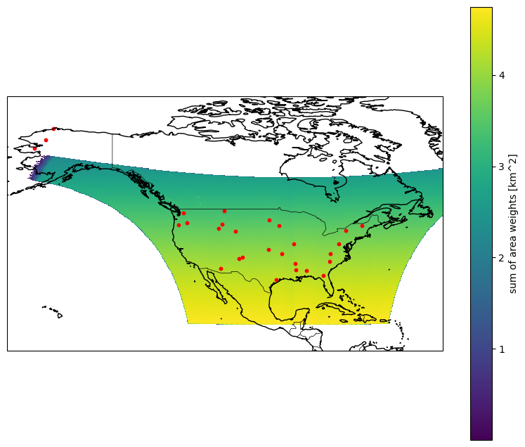
Plot our points with data
ds = plan . open_dataset ( 2 , open_method = tempo )
open_method: {'xarray_open': 'dataset', 'merge': ['/', '/product'], 'open_kwargs': {'chunks': {}, 'engine': 'h5netcdf', 'decode_timedelta': False}, 'coords': 'auto', 'set_coords': True, 'dim_renames': None, 'auto_align_phony_dims': None, 'merge_kwargs': {}}
Geolocation auto detected with cf_xarray: ('longitude', 'latitude') — lon dims=('longitude',), lat dims=('latitude',); time dim='time' (1 step(s))
Points columns used: y='lat', x='lon', time='time'
ds [ "vertical_column_troposphere" ] . units
import matplotlib.pyplot as plt
import cartopy.crs as ccrs
import cartopy.feature as cfeature
fig = plt . figure ( figsize = ( 10 , 8 ))
ds_plot = ds . weight . coarsen ( latitude = 10 , longitude = 10 , boundary = "trim" ) . mean ()
ax = plt . axes ( projection = ccrs . PlateCarree ())
# plot xarray field
ds_plot . plot (
ax = ax ,
transform = ccrs . PlateCarree (),
cmap = "viridis" ,
add_colorbar = True
)
# coastlines
ax . coastlines ( resolution = "50m" , linewidth = 1 )
# optional: borders
ax . add_feature ( cfeature . BORDERS , linewidth = 0.5 )
# plot dataframe points
ax . scatter (
df [ "lon" ],
df [ "lat" ],
color = "red" ,
s = 10 ,
transform = ccrs . PlateCarree (),
label = "points"
)
# zoom to North America
ax . set_extent ([ - 170 , - 50 , 10 , 80 ], crs = ccrs . PlateCarree ())
plt . show ()
TEMPO_O3TOT_L2
This is level 2 swath data. Let's take a look at how to get some matchups. The granule planning takes awhile so let's start with a few points.
import pandas as pd
url = (
"https://raw.githubusercontent.com/"
"fish-pace/point-collocation/main/"
"examples/fixtures/points_1000_usa.csv"
)
df_points = pd . read_csv (
url ,
parse_dates = [ "time" ]
)
df = df_points [
( df_points [ "time" ] . dt . year == 2024 ) &
( df_points [ "land" ] == True ) &
( df_points [ "lon" ] < - 60 ) &
( df_points [ "lon" ] > - 100 )
]
print ( len ( df ))
df . head ()
lat
lon
time
land
22
32.033815
-87.504205
2024-03-12 19:18:24
True
127
36.649735
-80.935069
2024-04-24 22:48:36
True
138
29.592103
-95.889008
2024-03-30 03:06:23
True
159
37.789200
-98.045855
2024-01-26 18:04:05
True
161
44.349757
-72.301856
2024-06-13 10:50:15
True
Get the plan
%% time
import point_collocation as pc
short_name = "TEMPO_O3TOT_L2"
plan = pc . plan (
df ,
data_source = "earthaccess" ,
source_kwargs = {
"short_name" : short_name ,
"version" : "V03"
},
time_buffer = "1h"
)
plan . summary ( n = 1 )
Plan: 15 points → 12 unique granule(s)
  Points with 0 matches : 9
  Points with >1 matches: 4
  Time buffer: 0 days 01:00:00

First 1 point(s):
  [22] lat=32.0338, lon=-87.5042, time=2024-03-12 19:18:24: 1 match(es)
    → https://data.asdc.earthdata.nasa.gov/asdc-prod-protected/TEMPO/TEMPO_O3TOT_L2_V03/2024.03.12/TEMPO_O3TOT_L2_V03_20240312T190833Z_S010G04.nc
CPU times: user 2.76 s, sys: 277 ms, total: 3.04 s
Wall time: 24.2 s
Take a look at the granules
These are grouped netcdfs and we need to figure out what groups we need and variable names.
ds = plan . open_dataset ( 0 , open_method = "datatree" )
ds
open_method: {'xarray_open': 'datatree', 'open_kwargs': {'chunks': {}, 'engine': 'h5netcdf', 'decode_timedelta': False}, 'merge': None, 'coords': 'auto', 'set_coords': True, 'dim_renames': None, 'auto_align_phony_dims': None}
Geolocation: could not detect lat/lon in dataset — no geolocation variables found. Expected one of the following (lon, lat) name pairs in ds.coords or ds.data_vars: [('lon', 'lat'), ('longitude', 'latitude'), ('Longitude', 'Latitude'), ('LONGITUDE', 'LATITUDE')]. Specify coords explicitly via open_method={'coords': {'lat': '...', 'lon': '...'}}.
<xarray.DataTree>
Group: /
│   Dimensions:      (xtrack: 2048, mirror_step: 131)
│   Coordinates:
│     * xtrack       (xtrack) int32 8kB 0 1 2 3 4 5 ... 2043 2044 2045 2046 2047
│     * mirror_step  (mirror_step) int32 524B 132 133 134 135 ... 259 260 261 262
│   Attributes: (12/34)
│       time_reference:                   1980-01-06T00:00:00Z
│       scan_num:                         1
│       granule_num:                      2
│       time_coverage_start:              2024-01-03T12:59:34Z
│       time_coverage_end:                2024-01-03T13:06:11Z
│       time_coverage_start_since_epoch:  1388321992.512726
│       ...                               ...
│       title:                            TEMPO Level 2 total ozone product
│       collection_shortname:             TEMPO_O3TOT_L2
│       collection_version:               1
│       keywords:                         EARTH SCIENCE>ATMOSPHERE>ATMOSPHERIC CH...
│       summary:                          Total ozone Level 2 files provide ozone...
│       coremetadata:                     \nGROUP                  = INVENTORYMET...
├── Group: /product
│       Dimensions:               (mirror_step: 131, xtrack: 2048)
│       Data variables:
│           column_amount_o3      (mirror_step, xtrack) float32 1MB dask.array<chunksize=(131, 2048), meta=np.ndarray>
│           radiative_cloud_frac  (mirror_step, xtrack) float32 1MB dask.array<chunksize=(131, 2048), meta=np.ndarray>
│           fc                    (mirror_step, xtrack) float32 1MB dask.array<chunksize=(131, 2048), meta=np.ndarray>
│           quality_flag          (mirror_step, xtrack) int32 1MB dask.array<chunksize=(131, 2048), meta=np.ndarray>
│           o3_below_cloud        (mirror_step, xtrack) float32 1MB dask.array<chunksize=(131, 2048), meta=np.ndarray>
│           so2_index             (mirror_step, xtrack) float32 1MB dask.array<chunksize=(131, 2048), meta=np.ndarray>
│           uv_aerosol_index      (mirror_step, xtrack) float32 1MB dask.array<chunksize=(131, 2048), meta=np.ndarray>
├── Group: /geolocation
│       Dimensions:                 (mirror_step: 131, xtrack: 2048, corner: 4)
│       Coordinates:
│           time                    (mirror_step) datetime64[ns] 1kB dask.array<chunksize=(131,), meta=np.ndarray>
│           latitude                (mirror_step, xtrack) float32 1MB dask.array<chunksize=(131, 2048), meta=np.ndarray>
│           longitude               (mirror_step, xtrack) float32 1MB dask.array<chunksize=(131, 2048), meta=np.ndarray>
│       Dimensions without coordinates: corner
│       Data variables:
│           latitude_bounds         (mirror_step, xtrack, corner) float32 4MB dask.array<chunksize=(131, 2048, 4), meta=np.ndarray>
│           longitude_bounds        (mirror_step, xtrack, corner) float32 4MB dask.array<chunksize=(131, 2048, 4), meta=np.ndarray>
│           solar_zenith_angle      (mirror_step, xtrack) float32 1MB dask.array<chunksize=(131, 2048), meta=np.ndarray>
│           solar_azimuth_angle     (mirror_step, xtrack) float32 1MB dask.array<chunksize=(131, 2048), meta=np.ndarray>
│           viewing_zenith_angle    (mirror_step, xtrack) float32 1MB dask.array<chunksize=(131, 2048), meta=np.ndarray>
│           viewing_azimuth_angle   (mirror_step, xtrack) float32 1MB dask.array<chunksize=(131, 2048), meta=np.ndarray>
│           relative_azimuth_angle  (mirror_step, xtrack) float32 1MB dask.array<chunksize=(131, 2048), meta=np.ndarray>
├── Group: /support_data
│       Dimensions:                        (mirror_step: 131, xtrack: 2048,
│                                           wavelength: 12, layer: 11)
│       Dimensions without coordinates: wavelength, layer
│       Data variables: (12/21)
│           ground_pixel_quality_flag      (mirror_step, xtrack) int32 1MB dask.array<chunksize=(131, 2048), meta=np.ndarray>
│           lut_wavelength                 (wavelength) float32 48B dask.array<chunksize=(12,), meta=np.ndarray>
│           cloud_pressure                 (mirror_step, xtrack) float32 1MB dask.array<chunksize=(131, 2048), meta=np.ndarray>
│           terrain_pressure               (mirror_step, xtrack) float32 1MB dask.array<chunksize=(131, 2048), meta=np.ndarray>
│           terrain_height                 (mirror_step, xtrack) float32 1MB dask.array<chunksize=(131, 2048), meta=np.ndarray>
│           algorithm_flags                (mirror_step, xtrack) int32 1MB dask.array<chunksize=(131, 2048), meta=np.ndarray>
│           ...                             ...
│           step_2_N_value_residual        (mirror_step, xtrack, wavelength) float32 13MB dask.array<chunksize=(1, 128, 12), meta=np.ndarray>
│           ozone_sensitivity_ratio        (mirror_step, xtrack, wavelength) float32 13MB dask.array<chunksize=(1, 128, 12), meta=np.ndarray>
│           temp_sensitivity_ratio         (mirror_step, xtrack, wavelength) float32 13MB dask.array<chunksize=(1, 128, 12), meta=np.ndarray>
│           step1_o3                       (mirror_step, xtrack) float32 1MB dask.array<chunksize=(131, 2048), meta=np.ndarray>
│           step2_o3                       (mirror_step, xtrack) float32 1MB dask.array<chunksize=(131, 2048), meta=np.ndarray>
│           cal_adjustment                 (xtrack, wavelength) float32 98kB dask.array<chunksize=(2048, 12), meta=np.ndarray>
└── Group: /qa_statistics Groups: (4)
Dimensions: xtrack : 2048mirror_step : 131
Data variables: (7)
column_amount_o3
(mirror_step, xtrack)
float32
dask.array<chunksize=(131, 2048), meta=np.ndarray>
comment : best total ozone solution units : DU valid_min : 50.0 valid_max : 700.0 Array Chunk Bytes 1.02 MiB 1.02 MiB Shape (131, 2048) (131, 2048) Dask graph 1 chunks in 2 graph layers Data type float32 numpy.ndarray
2048 131
radiative_cloud_frac
(mirror_step, xtrack)
float32
dask.array<chunksize=(131, 2048), meta=np.ndarray>
comment : cloud radiance fraction = fc*Ic331/Im331 valid_min : 0.0 valid_max : 1.0 Array Chunk Bytes 1.02 MiB 1.02 MiB Shape (131, 2048) (131, 2048) Dask graph 1 chunks in 2 graph layers Data type float32 numpy.ndarray
2048 131
fc
(mirror_step, xtrack)
float32
dask.array<chunksize=(131, 2048), meta=np.ndarray>
comment : effective cloud fraction (mixed LER model) valid_min : 0.0 valid_max : 1.0 Array Chunk Bytes 1.02 MiB 1.02 MiB Shape (131, 2048) (131, 2048) Dask graph 1 chunks in 2 graph layers Data type float32 numpy.ndarray
2048 131
quality_flag
(mirror_step, xtrack)
int32
dask.array<chunksize=(131, 2048), meta=np.ndarray>
comment : quality flags valid_min : 0 valid_max : 65534 flag_meanings : good_sample glint_contamination SZA>84 360_residual>threshold residual_at_unused_ozone_wavelenth>4sigma SOI>4sigma non-convergence abs(residual)>16.0(fatal) row_anomaly_error missing_TEMPO_cloud_pressure geolocation_error SZA>88 missing_input_radiance error_input_radiance warning_input_radiance missing_input_irradiance error_input_irradiance warning_input_irradiance flag_values : [ 0 1 2 3 4 5 6 7 8 128 256 5121024 2048 4096 8192 16384 32768] Array Chunk Bytes 1.02 MiB 1.02 MiB Shape (131, 2048) (131, 2048) Dask graph 1 chunks in 2 graph layers Data type int32 numpy.ndarray
2048 131
o3_below_cloud
(mirror_step, xtrack)
float32
dask.array<chunksize=(131, 2048), meta=np.ndarray>
comment : ozone below fractional cloud units : DU valid_min : 0.0 valid_max : 100.0 Array Chunk Bytes 1.02 MiB 1.02 MiB Shape (131, 2048) (131, 2048) Dask graph 1 chunks in 2 graph layers Data type float32 numpy.ndarray
2048 131
so2_index
(mirror_step, xtrack)
float32
dask.array<chunksize=(131, 2048), meta=np.ndarray>
comment : SO2 index valid_min : -300.0 valid_max : 300.0 Array Chunk Bytes 1.02 MiB 1.02 MiB Shape (131, 2048) (131, 2048) Dask graph 1 chunks in 2 graph layers Data type float32 numpy.ndarray
2048 131
uv_aerosol_index
(mirror_step, xtrack)
float32
dask.array<chunksize=(131, 2048), meta=np.ndarray>
comment : UV aerosol index valid_min : -30.0 valid_max : 30.0 Array Chunk Bytes 1.02 MiB 1.02 MiB Shape (131, 2048) (131, 2048) Dask graph 1 chunks in 2 graph layers Data type float32 numpy.ndarray
2048 131
Dimensions: xtrack : 2048mirror_step : 131corner : 4
Coordinates: (3)
time
(mirror_step)
datetime64[ns]
dask.array<chunksize=(131,), meta=np.ndarray>
standard_name : time comment : exposure start time valid_min : 0.0 valid_max : 10000000000.0 Array Chunk Bytes 1.02 kiB 1.02 kiB Shape (131,) (131,) Dask graph 1 chunks in 2 graph layers Data type datetime64[ns] numpy.ndarray
131 1
latitude
(mirror_step, xtrack)
float32
dask.array<chunksize=(131, 2048), meta=np.ndarray>
standard_name : latitude comment : latitude at pixel center units : degrees_north valid_min : -90.0 valid_max : 90.0 bounds : latitude_bounds Array Chunk Bytes 1.02 MiB 1.02 MiB Shape (131, 2048) (131, 2048) Dask graph 1 chunks in 2 graph layers Data type float32 numpy.ndarray
2048 131
longitude
(mirror_step, xtrack)
float32
dask.array<chunksize=(131, 2048), meta=np.ndarray>
standard_name : longitude comment : longitude at pixel center units : degrees_east valid_min : -180.0 valid_max : 180.0 bounds : longitude_bounds Array Chunk Bytes 1.02 MiB 1.02 MiB Shape (131, 2048) (131, 2048) Dask graph 1 chunks in 2 graph layers Data type float32 numpy.ndarray
2048 131
Data variables: (7)
latitude_bounds
(mirror_step, xtrack, corner)
float32
dask.array<chunksize=(131, 2048, 4), meta=np.ndarray>
comment : latitude at pixel corners (sw,se,ne,nw) valid_min : -90.0 valid_max : 90.0 Array Chunk Bytes 4.09 MiB 4.09 MiB Shape (131, 2048, 4) (131, 2048, 4) Dask graph 1 chunks in 2 graph layers Data type float32 numpy.ndarray
4 2048 131
longitude_bounds
(mirror_step, xtrack, corner)
float32
dask.array<chunksize=(131, 2048, 4), meta=np.ndarray>
comment : longitude at pixel corners (sw,se,ne,nw) valid_min : -180.0 valid_max : 180.0 Array Chunk Bytes 4.09 MiB 4.09 MiB Shape (131, 2048, 4) (131, 2048, 4) Dask graph 1 chunks in 2 graph layers Data type float32 numpy.ndarray
4 2048 131
solar_zenith_angle
(mirror_step, xtrack)
float32
dask.array<chunksize=(131, 2048), meta=np.ndarray>
comment : solar zenith angle at pixel center units : degrees valid_min : 0.0 valid_max : 180.0 Array Chunk Bytes 1.02 MiB 1.02 MiB Shape (131, 2048) (131, 2048) Dask graph 1 chunks in 2 graph layers Data type float32 numpy.ndarray
2048 131
solar_azimuth_angle
(mirror_step, xtrack)
float32
dask.array<chunksize=(131, 2048), meta=np.ndarray>
comment : solar azimuth angle at pixel center units : degrees valid_min : -180.0 valid_max : 180.0 Array Chunk Bytes 1.02 MiB 1.02 MiB Shape (131, 2048) (131, 2048) Dask graph 1 chunks in 2 graph layers Data type float32 numpy.ndarray
2048 131
viewing_zenith_angle
(mirror_step, xtrack)
float32
dask.array<chunksize=(131, 2048), meta=np.ndarray>
comment : viewing zenith angle at pixel center units : degrees valid_min : 0.0 valid_max : 180.0 Array Chunk Bytes 1.02 MiB 1.02 MiB Shape (131, 2048) (131, 2048) Dask graph 1 chunks in 2 graph layers Data type float32 numpy.ndarray
2048 131
viewing_azimuth_angle
(mirror_step, xtrack)
float32
dask.array<chunksize=(131, 2048), meta=np.ndarray>
comment : viewing azimuth angle at pixel center units : degrees valid_min : -180.0 valid_max : 180.0 Array Chunk Bytes 1.02 MiB 1.02 MiB Shape (131, 2048) (131, 2048) Dask graph 1 chunks in 2 graph layers Data type float32 numpy.ndarray
2048 131
relative_azimuth_angle
(mirror_step, xtrack)
float32
dask.array<chunksize=(131, 2048), meta=np.ndarray>
comment : relative azimuth angle (sun + 180 - view) units : degrees valid_min : -180.0 valid_max : 180.0 Array Chunk Bytes 1.02 MiB 1.02 MiB Shape (131, 2048) (131, 2048) Dask graph 1 chunks in 2 graph layers Data type float32 numpy.ndarray
2048 131
Dimensions: xtrack : 2048mirror_step : 131wavelength : 12layer : 11
Data variables: (21)
ground_pixel_quality_flag
(mirror_step, xtrack)
int32
dask.array<chunksize=(131, 2048), meta=np.ndarray>
comment : ground pixel quality flag valid_min : 0 valid_max : 65534 flag_meanings : shallow_ocean land shallow_inland_water shoreline intermittent_water deep_inland_water continental_shelf_ocean deep_ocean land_water_error sun_glint_possibility solar_eclipse_possibility goelocation_error flag_values : [ 0 1 2 3 4 5 6 7 15 16 32 64] Array Chunk Bytes 1.02 MiB 1.02 MiB Shape (131, 2048) (131, 2048) Dask graph 1 chunks in 2 graph layers Data type int32 numpy.ndarray
2048 131
lut_wavelength
(wavelength)
float32
dask.array<chunksize=(12,), meta=np.ndarray>
comment : lookup table wavelength units : nm valid_min : 300.0 valid_max : 400.0 Array Chunk Bytes 48 B 48 B Shape (12,) (12,) Dask graph 1 chunks in 2 graph layers Data type float32 numpy.ndarray
12 1
cloud_pressure
(mirror_step, xtrack)
float32
dask.array<chunksize=(131, 2048), meta=np.ndarray>
comment : effective cloud pressure units : hPA valid_min : 0.0 valid_max : 1013.25 Array Chunk Bytes 1.02 MiB 1.02 MiB Shape (131, 2048) (131, 2048) Dask graph 1 chunks in 2 graph layers Data type float32 numpy.ndarray
2048 131
terrain_pressure
(mirror_step, xtrack)
float32
dask.array<chunksize=(131, 2048), meta=np.ndarray>
comment : terrain pressure units : hPA valid_min : 0.0 valid_max : 1013.25 Array Chunk Bytes 1.02 MiB 1.02 MiB Shape (131, 2048) (131, 2048) Dask graph 1 chunks in 2 graph layers Data type float32 numpy.ndarray
2048 131
terrain_height
(mirror_step, xtrack)
float32
dask.array<chunksize=(131, 2048), meta=np.ndarray>
comment : terrain height units : m valid_min : -200 valid_max : 10000 Array Chunk Bytes 1.02 MiB 1.02 MiB Shape (131, 2048) (131, 2048) Dask graph 1 chunks in 2 graph layers Data type float32 numpy.ndarray
2048 131
algorithm_flags
(mirror_step, xtrack)
int32
dask.array<chunksize=(131, 2048), meta=np.ndarray>
comment : algorithm flags valid_min : 0 valid_max : 13 flag_meanings : skipped standard adjusted_for_profile_shape based_on_C-pair(331_and_360 nm) flag_values : [ 0 1 2 3 10] Array Chunk Bytes 1.02 MiB 1.02 MiB Shape (131, 2048) (131, 2048) Dask graph 1 chunks in 2 graph layers Data type int32 numpy.ndarray
2048 131
a_priori_layer_o3
(mirror_step, xtrack, layer)
float32
dask.array<chunksize=(1, 128, 11), meta=np.ndarray>
comment : a priori ozone profile valid_min : 0.0 valid_max : 125.0 Array Chunk Bytes 11.26 MiB 5.50 kiB Shape (131, 2048, 11) (1, 128, 11) Dask graph 2096 chunks in 2 graph layers Data type float32 numpy.ndarray
11 2048 131
radiance_bpix_flag_accepted
(mirror_step, xtrack)
int32
dask.array<chunksize=(131, 2048), meta=np.ndarray>
comment : radiance bad pixel flag accepted valid_min : 0 valid_max : 65534 Array Chunk Bytes 1.02 MiB 1.02 MiB Shape (131, 2048) (131, 2048) Dask graph 1 chunks in 2 graph layers Data type int32 numpy.ndarray
2048 131
layer_efficiency
(mirror_step, xtrack, layer)
float32
dask.array<chunksize=(1, 128, 11), meta=np.ndarray>
comment : algorithmic layer efficiency valid_min : 0.0 valid_max : 10.0 Array Chunk Bytes 11.26 MiB 5.50 kiB Shape (131, 2048, 11) (1, 128, 11) Dask graph 2096 chunks in 2 graph layers Data type float32 numpy.ndarray
11 2048 131
dNdR
(mirror_step, xtrack, wavelength)
float32
dask.array<chunksize=(1, 128, 12), meta=np.ndarray>
comment : reflectivity sensitivity ratio valid_min : -200.0 valid_max : 0.0 Array Chunk Bytes 12.28 MiB 6.00 kiB Shape (131, 2048, 12) (1, 128, 12) Dask graph 2096 chunks in 2 graph layers Data type float32 numpy.ndarray
12 2048 131
N_value
(mirror_step, xtrack, wavelength)
float32
dask.array<chunksize=(1, 128, 12), meta=np.ndarray>
comment : measured N-value valid_min : 0.0 valid_max : 600.0 Array Chunk Bytes 12.28 MiB 6.00 kiB Shape (131, 2048, 12) (1, 128, 12) Dask graph 2096 chunks in 2 graph layers Data type float32 numpy.ndarray
12 2048 131
surface_reflectivity_at_331nm
(mirror_step, xtrack)
float32
dask.array<chunksize=(131, 2048), meta=np.ndarray>
comment : effective surface reflectivity at 331 nm units : percent valid_min : -15.0 valid_max : 115.0 Array Chunk Bytes 1.02 MiB 1.02 MiB Shape (131, 2048) (131, 2048) Dask graph 1 chunks in 2 graph layers Data type float32 numpy.ndarray
2048 131
surface_reflectivity_at_360nm
(mirror_step, xtrack)
float32
dask.array<chunksize=(131, 2048), meta=np.ndarray>
comment : effective surface reflectivity at 360 nm units : percent valid_min : -15.0 valid_max : 115.0 Array Chunk Bytes 1.02 MiB 1.02 MiB Shape (131, 2048) (131, 2048) Dask graph 1 chunks in 2 graph layers Data type float32 numpy.ndarray
2048 131
N_value_residual
(mirror_step, xtrack, wavelength)
float32
dask.array<chunksize=(1, 128, 12), meta=np.ndarray>
comment : N-value residual valid_min : -32.0 valid_max : 32.0 Array Chunk Bytes 12.28 MiB 6.00 kiB Shape (131, 2048, 12) (1, 128, 12) Dask graph 2096 chunks in 2 graph layers Data type float32 numpy.ndarray
12 2048 131
step_1_N_value_residual
(mirror_step, xtrack, wavelength)
float32
dask.array<chunksize=(1, 128, 12), meta=np.ndarray>
comment : step 1 N-value residual valid_min : -32.0 valid_max : 32.0 Array Chunk Bytes 12.28 MiB 6.00 kiB Shape (131, 2048, 12) (1, 128, 12) Dask graph 2096 chunks in 2 graph layers Data type float32 numpy.ndarray
12 2048 131
step_2_N_value_residual
(mirror_step, xtrack, wavelength)
float32
dask.array<chunksize=(1, 128, 12), meta=np.ndarray>
comment : step 2 N-value residual valid_min : -32.0 valid_max : 32.0 Array Chunk Bytes 12.28 MiB 6.00 kiB Shape (131, 2048, 12) (1, 128, 12) Dask graph 2096 chunks in 2 graph layers Data type float32 numpy.ndarray
12 2048 131
ozone_sensitivity_ratio
(mirror_step, xtrack, wavelength)
float32
dask.array<chunksize=(1, 128, 12), meta=np.ndarray>
comment : ozone sensitivity ratio, dN/dOmega valid_min : 0.0 valid_max : 1.0 Array Chunk Bytes 12.28 MiB 6.00 kiB Shape (131, 2048, 12) (1, 128, 12) Dask graph 2096 chunks in 2 graph layers Data type float32 numpy.ndarray
12 2048 131
temp_sensitivity_ratio
(mirror_step, xtrack, wavelength)
float32
dask.array<chunksize=(1, 128, 12), meta=np.ndarray>
comment : ozone weighted temperature sensitivity ratio, dN/dT valid_min : 0.0 valid_max : 1.0 Array Chunk Bytes 12.28 MiB 6.00 kiB Shape (131, 2048, 12) (1, 128, 12) Dask graph 2096 chunks in 2 graph layers Data type float32 numpy.ndarray
12 2048 131
step1_o3
(mirror_step, xtrack)
float32
dask.array<chunksize=(131, 2048), meta=np.ndarray>
comment : step 1 ozone solution units : DU valid_min : 50.0 valid_max : 700.0 Array Chunk Bytes 1.02 MiB 1.02 MiB Shape (131, 2048) (131, 2048) Dask graph 1 chunks in 2 graph layers Data type float32 numpy.ndarray
2048 131
step2_o3
(mirror_step, xtrack)
float32
dask.array<chunksize=(131, 2048), meta=np.ndarray>
comment : step 2 ozone solution units : DU valid_min : 50.0 valid_max : 700.0 Array Chunk Bytes 1.02 MiB 1.02 MiB Shape (131, 2048) (131, 2048) Dask graph 1 chunks in 2 graph layers Data type float32 numpy.ndarray
2048 131
cal_adjustment
(xtrack, wavelength)
float32
dask.array<chunksize=(2048, 12), meta=np.ndarray>
comment : calibration adjustment valid_min : -10.0 valid_max : 10.0 Array Chunk Bytes 96.00 kiB 96.00 kiB Shape (2048, 12) (2048, 12) Dask graph 1 chunks in 2 graph layers Data type float32 numpy.ndarray
12 2048
Dimensions: xtrack : 2048mirror_step : 131
Coordinates: (2)
Attributes: (34)
time_reference : 1980-01-06T00:00:00Z scan_num : 1 granule_num : 2 time_coverage_start : 2024-01-03T12:59:34Z time_coverage_end : 2024-01-03T13:06:11Z time_coverage_start_since_epoch : 1388321992.512726 time_coverage_end_since_epoch : 1388322389.4111006 product_type : O3TOT processing_level : 2 processing_version : 3 sdpc_version : TEMPO_SDPC_v4.4.2 geospatial_bounds : POLYGON((58.7460 -63.7219,54.9606 -66.7865,50.7340 -69.3919,46.0275 -71.6021,41.2245 -73.3336,35.7360 -74.8531,29.8413 -76.0882,23.4120 -77.0890,17.2992 -77.7607,17.3834 -71.6776,21.3196 -71.0525,25.0933 -70.3146,28.6897 -69.4649,32.2082 -68.4707,35.5012 -67.3664,38.6396 -66.1259,41.6019 -64.7509,44.3806 -63.2414,46.9641 -61.6037,49.3638 -59.8332,51.7108 -57.8152,53.7180 -55.8028,55.6668 -53.5377,57.4343 -51.1466,59.1001 -48.5181,60.5875 -45.7741,59.5539 -55.2095,58.7763 -63.6414,58.7460 -63.7219)) geospatial_bounds_crs : EPSG:4326 geospatial_lon_min : -77.76071 geospatial_lon_max : -45.774143 geospatial_lat_min : 17.299183 geospatial_lat_max : 60.587494 input_files : TEMPO_RAD_L1_V03_20240103T125934Z_S001G02.nc, TEMPO_IRR_L1_V03_20231228T053116Z.nc, TEMPO_CLDO4_L2_V03_20240103T125934Z_S001G02.nc local_granule_id : TEMPO_O3TOT_L2_V03_20240103T125934Z_S001G02.nc version_id : 3 production_date_time : 2024-08-07T08:06:32.318 UTC-0400 day_of_year : 3 project : TEMPO platform : Intelsat 40e source : UV-VIS hyperspectral imaging institution : Smithsonian Astrophysical Observatory creator_url : http://tempo.si.edu Conventions : CF-1.6, ACDD-1.3 title : TEMPO Level 2 total ozone product collection_shortname : TEMPO_O3TOT_L2 collection_version : 1 keywords : EARTH SCIENCE>ATMOSPHERE>ATMOSPHERIC CHEMISTRY>OXYGEN COMPOUNDS>OZONE summary : Total ozone Level 2 files provide ozone information at TEMPO’s native spatial resolution, ~10 km^2 at the center of the Field of Regard (FOR), for individual granules. Each granule covers the entire North-South TEMPO FOR but only a portion of the East-West FOR. The files are provided in netCDF4 format, and contain information on total column ozone and some auxiliary derived and ancillary input parameters including N-values, effective Lambertian scene-reflectivity, UV aerosol index, SO2 index, cloud fraction, cloud pressure, ozone below clouds, terrain height, geolocation, solar and satellite viewing angles, and quality flags. The retrieval is based on the OMI TOMS V8.5 algorithm adapted for TEMPO. For further details, please refer to the ATBD. coremetadata :
GROUP = INVENTORYMETADATA
GROUPTYPE = MASTERGROUP
GROUP = ECSDATAGRANULE
OBJECT = LOCALGRANULEID
NUM_VAL = 1
VALUE = "TEMPO_O3TOT_L2_V03_20240103T125934Z_S001G02.nc"
END_OBJECT = LOCALGRANULEID
OBJECT = LOCALVERSIONID
NUM_VAL = 1
VALUE = ("RFC1321 MD5 = not yet calculated")
END_OBJECT = LOCALVERSIONID
OBJECT = PRODUCTIONDATETIME
NUM_VAL = 1
VALUE = "2024-08-07T12:06:32.000Z"
END_OBJECT = PRODUCTIONDATETIME
END_GROUP = ECSDATAGRANULE
GROUP = COLLECTIONDESCRIPTIONCLASS
OBJECT = SHORTNAME
NUM_VAL = 1
VALUE = "TEMPO_O3TOT_L2"
END_OBJECT = SHORTNAME
OBJECT = VERSIONID
NUM_VAL = 1
VALUE = (3)
END_OBJECT = VERSIONID
END_GROUP = COLLECTIONDESCRIPTIONCLASS
GROUP = INPUTGRANULE
OBJECT = INPUTPOINTER
NUM_VAL = 3
VALUE = ("TEMPO_RAD_L1_V03_20240103T125934Z_S001G02.nc", "TEMPO_IRR_L1_V03_20231228T053116Z.nc", "TEMPO_CLDO4_L2_V03_20240103T125934Z_S001G02.nc")
END_OBJECT = INPUTPOINTER
END_GROUP = INPUTGRANULE
GROUP = SPATIALDOMAINCONTAINER
GROUP = HORIZONTALSPATIALDOMAINCONTAINER
GROUP = GPOLYGON
OBJECT = GPOLYGONCONTAINER
CLASS = "1"
GROUP = GRINGPOINT
CLASS = "1"
OBJECT = GRINGPOINTLONGITUDE
NUM_VAL = 29
CLASS = "1"
VALUE = (-63.7218704223633, -66.7865447998047, -69.3919067382812, -71.6020584106445, -73.3336029052734, -74.8530654907227, -76.0881729125977, -77.0889892578125, -77.7607116699219, -71.6775817871094, -71.0524597167969, -70.3145980834961, -69.4649047851562, -68.470703125,
-67.3664245605469, -66.1259002685547, -64.7509384155273, -63.2413864135742, -61.6036949157715, -59.8332366943359, -57.8151702880859, -55.8027954101562, -53.5377426147461, -51.1465682983398, -48.5181427001953, -45.7741432189941, -55.2095375061035,
-63.6414031982422, -63.7218704223633)
END_OBJECT = GRINGPOINTLONGITUDE
OBJECT = GRINGPOINTLATITUDE
NUM_VAL = 29
CLASS = "1"
VALUE = (58.7460250854492, 54.9606132507324, 50.733959197998, 46.0275497436523, 41.2245101928711, 35.7360458374023, 29.8412837982178, 23.4120216369629, 17.2991828918457, 17.3833675384521, 21.3195819854736, 25.0932579040527, 28.6896781921387, 32.2081680297852,
35.5011901855469, 38.6395874023438, 41.6018981933594, 44.3806228637695, 46.9640960693359, 49.3638229370117, 51.710807800293, 53.7180252075195, 55.6668243408203, 57.4343490600586, 59.1000556945801, 60.5874938964844, 59.5538940429688, 58.7763061523438,
58.7460250854492)
END_OBJECT = GRINGPOINTLATITUDE
OBJECT = GRINGPOINTSEQUENCENO
NUM_VAL = 29
CLASS = "1"
VALUE = (1, 2, 3, 4, 5, 6, 7, 8, 9, 10, 11, 12, 13, 14, 15, 16, 17, 18, 19, 20, 21, 22, 23, 24, 25, 26, 27, 28, 29)
END_OBJECT = GRINGPOINTSEQUENCENO
END_GROUP = GRINGPOINT
GROUP = GRING
CLASS = "1"
OBJECT = EXCLUSIONGRINGFLAG
NUM_VAL = 1
VALUE = "N"
CLASS = "1"
END_OBJECT = EXCLUSIONGRINGFLAG
END_GROUP = GRING
END_OBJECT = GPOLYGONCONTAINER
END_GROUP = GPOLYGON
END_GROUP = HORIZONTALSPATIALDOMAINCONTAINER
END_GROUP = SPATIALDOMAINCONTAINER
GROUP = RANGEDATETIME
OBJECT = RANGEENDINGDATE
NUM_VAL = 1
VALUE = "2024-01-03"
END_OBJECT = RANGEENDINGDATE
OBJECT = RANGEENDINGTIME
NUM_VAL = 1
VALUE = "13:06:11"
END_OBJECT = RANGEENDINGTIME
OBJECT = RANGEBEGINNINGDATE
NUM_VAL = 1
VALUE = "2024-01-03"
END_OBJECT = RANGEBEGINNINGDATE
OBJECT = RANGEBEGINNINGTIME
NUM_VAL = 1
VALUE = "12:59:34"
END_OBJECT = RANGEBEGINNINGTIME
END_GROUP = RANGEDATETIME
GROUP = PGEVERSIONCLASS
OBJECT = PGEVERSION
NUM_VAL = 1
VALUE = ("2.2.1")
END_OBJECT = PGEVERSION
END_GROUP = PGEVERSIONCLASS
END_GROUP = INVENTORYMETADATA
END
Ok now we know the groups
We will make a open_method dictionary.
tempo_l2 = {
'xarray_open' : 'dataset' ,
'merge' : [ '/product' , '/geolocation' ],
'coords' : { 'lat' : 'latitude' , 'lon' : 'longitude' },
}
ds = plan . open_dataset ( 0 , open_method = tempo_l2 )
ds
open_method: {'xarray_open': 'dataset', 'merge': ['/product', '/geolocation'], 'coords': {'lat': 'latitude', 'lon': 'longitude'}, 'open_kwargs': {'chunks': {}, 'engine': 'h5netcdf', 'decode_timedelta': False}, 'set_coords': True, 'dim_renames': None, 'auto_align_phony_dims': None, 'merge_kwargs': {}}
Geolocation specified: ('longitude', 'latitude') — lon dims=('mirror_step', 'xtrack'), lat dims=('mirror_step', 'xtrack')
Points columns used: y='lat', x='lon', time='time'
<xarray.Dataset> Size: 24MB
Dimensions:                 (mirror_step: 131, xtrack: 2048, corner: 4)
Coordinates:
    time                    (mirror_step) datetime64[ns] 1kB dask.array<chunksize=(131,), meta=np.ndarray>
    latitude                (mirror_step, xtrack) float32 1MB dask.array<chunksize=(131, 2048), meta=np.ndarray>
    longitude               (mirror_step, xtrack) float32 1MB dask.array<chunksize=(131, 2048), meta=np.ndarray>
Dimensions without coordinates: mirror_step, xtrack, corner
Data variables: (12/14)
    column_amount_o3        (mirror_step, xtrack) float32 1MB dask.array<chunksize=(131, 2048), meta=np.ndarray>
    radiative_cloud_frac    (mirror_step, xtrack) float32 1MB dask.array<chunksize=(131, 2048), meta=np.ndarray>
    fc                      (mirror_step, xtrack) float32 1MB dask.array<chunksize=(131, 2048), meta=np.ndarray>
    quality_flag            (mirror_step, xtrack) int32 1MB dask.array<chunksize=(131, 2048), meta=np.ndarray>
    o3_below_cloud          (mirror_step, xtrack) float32 1MB dask.array<chunksize=(131, 2048), meta=np.ndarray>
    so2_index               (mirror_step, xtrack) float32 1MB dask.array<chunksize=(131, 2048), meta=np.ndarray>
    ...                      ...
    longitude_bounds        (mirror_step, xtrack, corner) float32 4MB dask.array<chunksize=(131, 2048, 4), meta=np.ndarray>
    solar_zenith_angle      (mirror_step, xtrack) float32 1MB dask.array<chunksize=(131, 2048), meta=np.ndarray>
    solar_azimuth_angle     (mirror_step, xtrack) float32 1MB dask.array<chunksize=(131, 2048), meta=np.ndarray>
    viewing_zenith_angle    (mirror_step, xtrack) float32 1MB dask.array<chunksize=(131, 2048), meta=np.ndarray>
    viewing_azimuth_angle   (mirror_step, xtrack) float32 1MB dask.array<chunksize=(131, 2048), meta=np.ndarray>
relative_azimuth_angle (mirror_step, xtrack) float32 1MB dask.array<chunksize=(131, 2048), meta=np.ndarray> Dimensions: mirror_step : 131xtrack : 2048corner : 4
Coordinates: (3)
time
(mirror_step)
datetime64[ns]
dask.array<chunksize=(131,), meta=np.ndarray>
standard_name : time comment : exposure start time valid_min : 0.0 valid_max : 10000000000.0
Array
Chunk
Bytes
1.02 kiB
1.02 kiB
Shape
(131,)
(131,)
Dask graph
1 chunks in 2 graph layers
Data type
datetime64[ns] numpy.ndarray
131
1
latitude
(mirror_step, xtrack)
float32
dask.array<chunksize=(131, 2048), meta=np.ndarray>
standard_name : latitude comment : latitude at pixel center units : degrees_north valid_min : -90.0 valid_max : 90.0 bounds : latitude_bounds
Array
Chunk
Bytes
1.02 MiB
1.02 MiB
Shape
(131, 2048)
(131, 2048)
Dask graph
1 chunks in 2 graph layers
Data type
float32 numpy.ndarray
2048
131
longitude
(mirror_step, xtrack)
float32
dask.array<chunksize=(131, 2048), meta=np.ndarray>
standard_name : longitude comment : longitude at pixel center units : degrees_east valid_min : -180.0 valid_max : 180.0 bounds : longitude_bounds
Array
Chunk
Bytes
1.02 MiB
1.02 MiB
Shape
(131, 2048)
(131, 2048)
Dask graph
1 chunks in 2 graph layers
Data type
float32 numpy.ndarray
2048
131
Data variables: (14)
column_amount_o3
(mirror_step, xtrack)
float32
dask.array<chunksize=(131, 2048), meta=np.ndarray>
comment : best total ozone solution units : DU valid_min : 50.0 valid_max : 700.0
Array
Chunk
Bytes
1.02 MiB
1.02 MiB
Shape
(131, 2048)
(131, 2048)
Dask graph
1 chunks in 2 graph layers
Data type
float32 numpy.ndarray
2048
131
radiative_cloud_frac
(mirror_step, xtrack)
float32
dask.array<chunksize=(131, 2048), meta=np.ndarray>
comment : cloud radiance fraction = fc*Ic331/Im331 valid_min : 0.0 valid_max : 1.0
Array
Chunk
Bytes
1.02 MiB
1.02 MiB
Shape
(131, 2048)
(131, 2048)
Dask graph
1 chunks in 2 graph layers
Data type
float32 numpy.ndarray
2048
131
fc
(mirror_step, xtrack)
float32
dask.array<chunksize=(131, 2048), meta=np.ndarray>
comment : effective cloud fraction (mixed LER model) valid_min : 0.0 valid_max : 1.0
Array
Chunk
Bytes
1.02 MiB
1.02 MiB
Shape
(131, 2048)
(131, 2048)
Dask graph
1 chunks in 2 graph layers
Data type
float32 numpy.ndarray
2048
131
quality_flag
(mirror_step, xtrack)
int32
dask.array<chunksize=(131, 2048), meta=np.ndarray>
comment : quality flags valid_min : 0 valid_max : 65534 flag_meanings : good_sample glint_contamination SZA>84 360_residual>threshold residual_at_unused_ozone_wavelenth>4sigma SOI>4sigma non-convergence abs(residual)>16.0(fatal) row_anomaly_error missing_TEMPO_cloud_pressure geolocation_error SZA>88 missing_input_radiance error_input_radiance warning_input_radiance missing_input_irradiance error_input_irradiance warning_input_irradiance flag_values : [ 0 1 2 3 4 5 6 7 8 128 256 512
1024 2048 4096 8192 16384 32768]
Array
Chunk
Bytes
1.02 MiB
1.02 MiB
Shape
(131, 2048)
(131, 2048)
Dask graph
1 chunks in 2 graph layers
Data type
int32 numpy.ndarray
2048
131
o3_below_cloud
(mirror_step, xtrack)
float32
dask.array<chunksize=(131, 2048), meta=np.ndarray>
comment : ozone below fractional cloud units : DU valid_min : 0.0 valid_max : 100.0
Array
Chunk
Bytes
1.02 MiB
1.02 MiB
Shape
(131, 2048)
(131, 2048)
Dask graph
1 chunks in 2 graph layers
Data type
float32 numpy.ndarray
2048
131
so2_index
(mirror_step, xtrack)
float32
dask.array<chunksize=(131, 2048), meta=np.ndarray>
comment : SO2 index valid_min : -300.0 valid_max : 300.0
Array
Chunk
Bytes
1.02 MiB
1.02 MiB
Shape
(131, 2048)
(131, 2048)
Dask graph
1 chunks in 2 graph layers
Data type
float32 numpy.ndarray
2048
131
uv_aerosol_index
(mirror_step, xtrack)
float32
dask.array<chunksize=(131, 2048), meta=np.ndarray>
comment : UV aerosol index valid_min : -30.0 valid_max : 30.0
Array
Chunk
Bytes
1.02 MiB
1.02 MiB
Shape
(131, 2048)
(131, 2048)
Dask graph
1 chunks in 2 graph layers
Data type
float32 numpy.ndarray
2048
131
latitude_bounds
(mirror_step, xtrack, corner)
float32
dask.array<chunksize=(131, 2048, 4), meta=np.ndarray>
comment : latitude at pixel corners (sw,se,ne,nw) valid_min : -90.0 valid_max : 90.0
Array
Chunk
Bytes
4.09 MiB
4.09 MiB
Shape
(131, 2048, 4)
(131, 2048, 4)
Dask graph
1 chunks in 2 graph layers
Data type
float32 numpy.ndarray
4
2048
131
longitude_bounds
(mirror_step, xtrack, corner)
float32
dask.array<chunksize=(131, 2048, 4), meta=np.ndarray>
comment : longitude at pixel corners (sw,se,ne,nw) valid_min : -180.0 valid_max : 180.0
Array
Chunk
Bytes
4.09 MiB
4.09 MiB
Shape
(131, 2048, 4)
(131, 2048, 4)
Dask graph
1 chunks in 2 graph layers
Data type
float32 numpy.ndarray
4
2048
131
solar_zenith_angle
(mirror_step, xtrack)
float32
dask.array<chunksize=(131, 2048), meta=np.ndarray>
comment : solar zenith angle at pixel center units : degrees valid_min : 0.0 valid_max : 180.0
Array
Chunk
Bytes
1.02 MiB
1.02 MiB
Shape
(131, 2048)
(131, 2048)
Dask graph
1 chunks in 2 graph layers
Data type
float32 numpy.ndarray
2048
131
solar_azimuth_angle
(mirror_step, xtrack)
float32
dask.array<chunksize=(131, 2048), meta=np.ndarray>
comment : solar azimuth angle at pixel center units : degrees valid_min : -180.0 valid_max : 180.0
Array
Chunk
Bytes
1.02 MiB
1.02 MiB
Shape
(131, 2048)
(131, 2048)
Dask graph
1 chunks in 2 graph layers
Data type
float32 numpy.ndarray
2048
131
viewing_zenith_angle
(mirror_step, xtrack)
float32
dask.array<chunksize=(131, 2048), meta=np.ndarray>
comment : viewing zenith angle at pixel center units : degrees valid_min : 0.0 valid_max : 180.0
Array
Chunk
Bytes
1.02 MiB
1.02 MiB
Shape
(131, 2048)
(131, 2048)
Dask graph
1 chunks in 2 graph layers
Data type
float32 numpy.ndarray
2048
131
viewing_azimuth_angle
(mirror_step, xtrack)
float32
dask.array<chunksize=(131, 2048), meta=np.ndarray>
comment : viewing azimuth angle at pixel center units : degrees valid_min : -180.0 valid_max : 180.0
Array
Chunk
Bytes
1.02 MiB
1.02 MiB
Shape
(131, 2048)
(131, 2048)
Dask graph
1 chunks in 2 graph layers
Data type
float32 numpy.ndarray
2048
131
relative_azimuth_angle
(mirror_step, xtrack)
float32
dask.array<chunksize=(131, 2048), meta=np.ndarray>
comment : relative azimuth angle (sun + 180 - view) units : degrees valid_min : -180.0 valid_max : 180.0
Array
Chunk
Bytes
1.02 MiB
1.02 MiB
Shape
(131, 2048)
(131, 2048)
Dask graph
1 chunks in 2 graph layers
Data type
float32 numpy.ndarray
2048
131
Now we get the matchups using this open_method dict
It is roughly 2 seconds per point. So roughly 5 hrs for 10,000 points.
%% time
res = pc . matchup ( plan ,
variables = [ "uv_aerosol_index" ],
open_method = tempo_l2 )
CPU times: user 10.1 s, sys: 691 ms, total: 10.8 s
Wall time: 25.5 s
(
res [[ 'lat' , 'lon' , 'time' , 'uv_aerosol_index' ]]
. dropna ( subset = [ 'uv_aerosol_index' ])
)
lat
lon
time
uv_aerosol_index
0
32.033815
-87.504205
2024-03-12 19:18:24
-2.219414
1
36.649735
-80.935069
2024-04-24 22:48:36
-2.591015
4
44.349757
-72.301856
2024-06-13 10:50:15
-1.152082
5
44.349757
-72.301856
2024-06-13 10:50:15
-1.889225
6
44.355987
-95.126999
2024-01-14 16:55:19
-2.514838
7
44.355987
-95.126999
2024-01-14 16:55:19
-2.738163
9
34.035328
-90.559024
2024-07-31 23:17:20
-2.717468
10
34.035328
-90.559024
2024-07-31 23:17:20
-2.282551
11
34.035328
-90.559024
2024-07-31 23:17:20
-1.936824
17
45.961109
-97.761663
2024-07-01 12:06:54
-1.305435
18
45.961109
-97.761663
2024-07-01 12:06:54
-1.612602
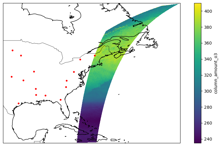
Here is a plot showing points and swaths
This is just one swath. The matchup routine finds the granules matching each point.
import matplotlib.pyplot as plt
import cartopy.crs as ccrs
import cartopy.feature as cfeature
var = ds [ "column_amount_o3" ]
fig = plt . figure ( figsize = ( 12 , 6 ))
ax = plt . axes ( projection = ccrs . PlateCarree ())
pcm = ax . pcolormesh (
ds [ "longitude" ],
ds [ "latitude" ],
var ,
shading = "auto" ,
transform = ccrs . PlateCarree ()
)
# plot dataframe points
ax . scatter (
df [ "lon" ],
df [ "lat" ],
color = "red" ,
s = 10 ,
transform = ccrs . PlateCarree (),
label = "points"
)
ax . coastlines ()
ax . add_feature ( cfeature . BORDERS , linewidth = 0.5 )
ax . set_xlabel ( "Longitude" )
ax . set_ylabel ( "Latitude" )
plt . colorbar ( pcm , ax = ax , label = var . name )
plt . show ()