![]()
MERRA-2
MERRA-2 (Modern-Era Retrospective analysis for Research and Applications, Version 2) is a global gap-free atmospheric reanalysis dataset from NASA that combines models and observations to produce a consistent, gridded record of Earth’s atmosphere over time. The dataset covers the period of 1980-present with the latency of ~3 weeks after the end of a month. It has a spatial grid of ~0.5° latitude × 0.625° longitude, hourly to monthly products and is 3D atmosphere (multiple heights).
Variables include:
- Meteorology: air temperature, winds, air pressure, humidity
- Surface: fluxes, precipitation, radiation
- Aerosols: dust, sea salt, black carbon, sulfate
- Land surface: soil temperature and moisture, greenness
We will get matchups for 2 data collections:
M2TMNXLND: monthly, gridded MERRA-2 land surface dataset providing soil moisture, soil temperature, snow, and land–atmosphere fluxes such as evaporation and runoff on a global grid.M2T3NVASM: 3-hour, gridded MERRA-2 dataset providing time-averaged 3D atmospheric variables (e.g., temperature, winds, humidity) on standard pressure levels.
Note: In a virtual machine in AWS us-west-2, where NASA cloud data is, the point matchups are fast. In Colab, say, your compute is not in the same data region nor provider, and the same matchups might take 10x longer.
Prerequisites
The examples here use NASA EarthData and you need to have an account with EarthData. Make sure you can login.
<earthaccess.auth.Auth at 0x7fb0cbd1bc20>
There are many MERRA-2 collections available
Chatbots are good ways to explore what they are.
import earthaccess
results = earthaccess.search_datasets(
    project = 'MERRA-2',
)
print(len(results))
for item in results[0:10]:
    summary = item.summary()
    print(summary["short-name"])
104
M2_TMAX_PM25
M2C0NXASM
M2C0NXCTM
M2C0NXLND
M2I1NXASM
M2I1NXINT
M2I1NXLFO
M2I3NXGAS
M2I3NVAER
M2I3NPASM
Get some sample points over land
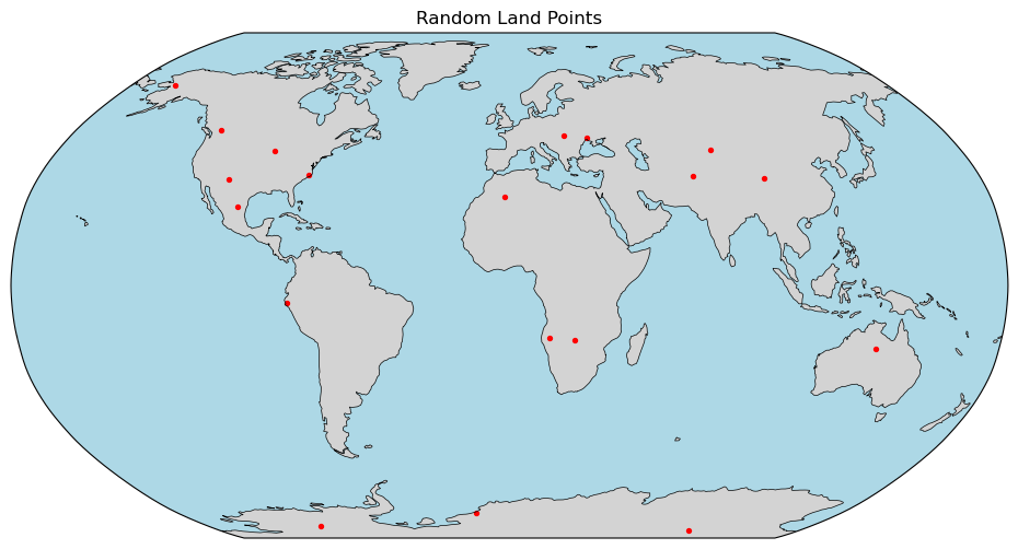
We will start with a land dataset so want points over land.
import pandas as pd
url = (
    "https://raw.githubusercontent.com/"
    "fish-pace/point-collocation/main/"
    "examples/fixtures/points_1000.csv"
)
df_points = pd.read_csv(
    url,
    parse_dates=["time"]
)
df = df_points[
    (df_points["time"].dt.year < 2018) &
    (df_points["time"].dt.year > 2014) &
    (df_points["land"] == True)
].reset_index(drop=True)
# Force all timestamps to noon UTC to avoid "midnight overlap" issues
df["time"] = df["time"].dt.normalize() + pd.Timedelta(hours=12)
print(len(df))
df.head()
19
| lat | lon | time | land | |
|---|---|---|---|---|
| 0 | -17.432469 | 24.018931 | 2015-08-22 12:00:00 | True |
| 1 | -16.707673 | 14.478041 | 2016-03-24 12:00:00 | True |
| 2 | -83.839933 | 111.134906 | 2015-05-06 12:00:00 | True |
| 3 | 65.250200 | -159.513009 | 2017-10-29 12:00:00 | True |
| 4 | 28.315760 | -1.839657 | 2016-12-14 12:00:00 | True |
Let's plot the points
import matplotlib.pyplot as plt
import cartopy.crs as ccrs
import cartopy.feature as cfeature

# create Robinson projection
proj = ccrs.Robinson()

fig = plt.figure(figsize=(12,6))
ax = plt.axes(projection=proj)

# add map features
ax.add_feature(cfeature.LAND, facecolor="lightgray")
ax.add_feature(cfeature.OCEAN, facecolor="lightblue")
ax.add_feature(cfeature.COASTLINE, linewidth=0.5)

# plot points
ax.scatter(
    df["lon"],
    df["lat"],
    s=8,
    color="red",
    transform=ccrs.PlateCarree()
)

ax.set_global()
plt.title("Random Land Points")
plt.show()
MERRA LAND
Create the granule plan
import point_collocation as pc
short_name="M2TMNXLND"
plan = pc.plan(
    df,
    data_source="earthaccess",
    source_kwargs={
        "short_name": short_name,
    }
)
plan.summary(n=2)
Plan: 19 points → 16 unique granule(s)
  Points with 0 matches : 0
  Points with >1 matches: 0
  Time buffer: 0 days 00:00:00

First 2 point(s):
  [0] lat=-17.4325, lon=24.0189, time=2015-08-22 12:00:00: 1 match(es)
    → https://data.gesdisc.earthdata.nasa.gov/data/MERRA2_MONTHLY/M2TMNXLND.5.12.4/2015/MERRA2_400.tavgM_2d_lnd_Nx.201508.nc4
  [1] lat=-16.7077, lon=14.4780, time=2016-03-24 12:00:00: 1 match(es)
    → https://data.gesdisc.earthdata.nasa.gov/data/MERRA2_MONTHLY/M2TMNXLND.5.12.4/2016/MERRA2_400.tavgM_2d_lnd_Nx.201603.nc4
[Collection: {'ShortName': 'M2TMNXLND', 'Version': '5.12.4'}
 Spatial coverage: {'HorizontalSpatialDomain': {'Geometry': {'BoundingRectangles': [{'WestBoundingCoordinate': -180.0, 'EastBoundingCoordinate': 180.0, 'NorthBoundingCoordinate': 90.0, 'SouthBoundingCoordinate': -90.0}]}}}
 Temporal coverage: {'RangeDateTime': {'BeginningDateTime': '2015-01-01T00:00:00.000Z', 'EndingDateTime': '2015-01-31T23:59:59.000Z'}}
 Size(MB): 18.402777671813965
 Data: ['https://data.gesdisc.earthdata.nasa.gov/data/MERRA2_MONTHLY/M2TMNXLND.5.12.4/2015/MERRA2_400.tavgM_2d_lnd_Nx.201501.nc4']]
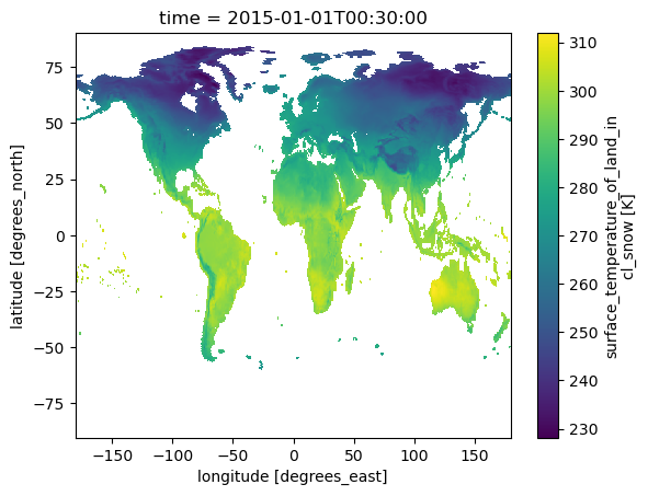
Let's plot a granule to see how it looks
There are many data variables. We will get
- TSURF surface temperature
- GWETROOT root zone wetness
- LAI leaf area index
open_method: {'xarray_open': 'dataset', 'open_kwargs': {'chunks': {}, 'engine': 'h5netcdf', 'decode_timedelta': False}, 'coords': 'auto', 'set_coords': True, 'dim_renames': None, 'auto_align_phony_dims': None, 'merge': None}
Geolocation auto detected with cf_xarray: ('lon', 'lat') — lon dims=('lon',), lat dims=('lat',); time dim='time' (1 step(s))
Points columns used: y='lat', x='lon', time='time'
CPU times: user 10.6 s, sys: 49.9 ms, total: 10.6 s
Wall time: 10.9 s
<xarray.Dataset> Size: 83MB
Dimensions:          (time: 1, lat: 361, lon: 576)
Coordinates:
  * time             (time) datetime64[ns] 8B 2015-01-01T00:30:00
  * lat              (lat) float64 3kB -90.0 -89.5 -89.0 ... 89.0 89.5 90.0
  * lon              (lon) float64 5kB -180.0 -179.4 -178.8 ... 178.8 179.4
Data variables: (12/100)
    BASEFLOW         (time, lat, lon) float32 832kB dask.array<chunksize=(1, 91, 144), meta=np.ndarray>
    ECHANGE          (time, lat, lon) float32 832kB dask.array<chunksize=(1, 91, 144), meta=np.ndarray>
    EVLAND           (time, lat, lon) float32 832kB dask.array<chunksize=(1, 91, 144), meta=np.ndarray>
    EVPINTR          (time, lat, lon) float32 832kB dask.array<chunksize=(1, 91, 144), meta=np.ndarray>
    EVPSBLN          (time, lat, lon) float32 832kB dask.array<chunksize=(1, 91, 144), meta=np.ndarray>
    EVPSOIL          (time, lat, lon) float32 832kB dask.array<chunksize=(1, 91, 144), meta=np.ndarray>
    ...               ...
    Var_TSOIL6       (time, lat, lon) float32 832kB dask.array<chunksize=(1, 91, 144), meta=np.ndarray>
    Var_TSURF        (time, lat, lon) float32 832kB dask.array<chunksize=(1, 91, 144), meta=np.ndarray>
    Var_TUNST        (time, lat, lon) float32 832kB dask.array<chunksize=(1, 91, 144), meta=np.ndarray>
    Var_TWLAND       (time, lat, lon) float32 832kB dask.array<chunksize=(1, 91, 144), meta=np.ndarray>
    Var_TWLT         (time, lat, lon) float32 832kB dask.array<chunksize=(1, 91, 144), meta=np.ndarray>
    Var_WCHANGE      (time, lat, lon) float32 832kB dask.array<chunksize=(1, 91, 144), meta=np.ndarray>
Attributes: (12/30)
    History:                           Original file generated: Mon Mar 23 22...
    Filename:                          MERRA2_400.tavgM_2d_lnd_Nx.201501.nc4
    Comment:                           GMAO filename: d5124_m2_jan10.tavg1_2d...
    Conventions:                       CF-1
    Institution:                       NASA Global Modeling and Assimilation ...
    References:                        http://gmao.gsfc.nasa.gov
    ...                                ...
    DataResolution:                    0.5 x 0.625
    Source:                            CVS tag: GEOSadas-5_12_4
    Contact:                           http://gmao.gsfc.nasa.gov
    identifier_product_doi:            10.5067/8S35XF81C28F
    RangeBeginningTime:                00:00:00.000000
RangeEndingTime: 23:59:59.000000- time: 1
- lat: 361
- lon: 576
- time(time)datetime64[ns]2015-01-01T00:30:00
- long_name :
- time
- time_increment :
- 60000
- begin_date :
- 20150101
- begin_time :
- 3000
- vmax :
- 1e+15
- vmin :
- -1e+15
- valid_range :
- [-1.e+15 1.e+15]
array(['2015-01-01T00:30:00.000000000'], dtype='datetime64[ns]')
- lat(lat)float64-90.0 -89.5 -89.0 ... 89.5 90.0
- long_name :
- latitude
- units :
- degrees_north
- vmax :
- 1e+15
- vmin :
- -1e+15
- valid_range :
- [-1.e+15 1.e+15]
array([-90. , -89.5, -89. , ..., 89. , 89.5, 90. ], shape=(361,))
- lon(lon)float64-180.0 -179.4 ... 178.8 179.4
- long_name :
- longitude
- units :
- degrees_east
- vmax :
- 1e+15
- vmin :
- -1e+15
- valid_range :
- [-1.e+15 1.e+15]
array([-180.   , -179.375, -178.75 , ...,  178.125,  178.75 ,  179.375],
      shape=(576,))
- BASEFLOW(time, lat, lon)float32dask.array<chunksize=(1, 91, 144), meta=np.ndarray>
- long_name :
- baseflow_flux
- units :
- kg m-2 s-1
- fmissing_value :
- 1e+15
- vmax :
- 1e+15
- vmin :
- -1e+15
- valid_range :
- [-1.e+15 1.e+15]
Array Chunk Bytes 812.25 kiB 51.19 kiB Shape (1, 361, 576) (1, 91, 144) Dask graph 16 chunks in 2 graph layers Data type float32 numpy.ndarray - ECHANGE(time, lat, lon)float32dask.array<chunksize=(1, 91, 144), meta=np.ndarray>
- long_name :
- rate_of_change_of_total_land_energy
- units :
- W m-2
- fmissing_value :
- 1e+15
- vmax :
- 1e+15
- vmin :
- -1e+15
- valid_range :
- [-1.e+15 1.e+15]
Array Chunk Bytes 812.25 kiB 51.19 kiB Shape (1, 361, 576) (1, 91, 144) Dask graph 16 chunks in 2 graph layers Data type float32 numpy.ndarray - EVLAND(time, lat, lon)float32dask.array<chunksize=(1, 91, 144), meta=np.ndarray>
- long_name :
- Evaporation_land
- units :
- kg m-2 s-1
- fmissing_value :
- 1e+15
- vmax :
- 1e+15
- vmin :
- -1e+15
- valid_range :
- [-1.e+15 1.e+15]
Array Chunk Bytes 812.25 kiB 51.19 kiB Shape (1, 361, 576) (1, 91, 144) Dask graph 16 chunks in 2 graph layers Data type float32 numpy.ndarray - EVPINTR(time, lat, lon)float32dask.array<chunksize=(1, 91, 144), meta=np.ndarray>
- long_name :
- interception_loss_energy_flux
- units :
- W m-2
- fmissing_value :
- 1e+15
- vmax :
- 1e+15
- vmin :
- -1e+15
- valid_range :
- [-1.e+15 1.e+15]
Array Chunk Bytes 812.25 kiB 51.19 kiB Shape (1, 361, 576) (1, 91, 144) Dask graph 16 chunks in 2 graph layers Data type float32 numpy.ndarray - EVPSBLN(time, lat, lon)float32dask.array<chunksize=(1, 91, 144), meta=np.ndarray>
- long_name :
- snow_ice_evaporation_energy_flux
- units :
- W m-2
- fmissing_value :
- 1e+15
- vmax :
- 1e+15
- vmin :
- -1e+15
- valid_range :
- [-1.e+15 1.e+15]
Array Chunk Bytes 812.25 kiB 51.19 kiB Shape (1, 361, 576) (1, 91, 144) Dask graph 16 chunks in 2 graph layers Data type float32 numpy.ndarray - EVPSOIL(time, lat, lon)float32dask.array<chunksize=(1, 91, 144), meta=np.ndarray>
- long_name :
- baresoil_evap_energy_flux
- units :
- W m-2
- fmissing_value :
- 1e+15
- vmax :
- 1e+15
- vmin :
- -1e+15
- valid_range :
- [-1.e+15 1.e+15]
Array Chunk Bytes 812.25 kiB 51.19 kiB Shape (1, 361, 576) (1, 91, 144) Dask graph 16 chunks in 2 graph layers Data type float32 numpy.ndarray - EVPTRNS(time, lat, lon)float32dask.array<chunksize=(1, 91, 144), meta=np.ndarray>
- long_name :
- transpiration_energy_flux
- units :
- W m-2
- fmissing_value :
- 1e+15
- vmax :
- 1e+15
- vmin :
- -1e+15
- valid_range :
- [-1.e+15 1.e+15]
Array Chunk Bytes 812.25 kiB 51.19 kiB Shape (1, 361, 576) (1, 91, 144) Dask graph 16 chunks in 2 graph layers Data type float32 numpy.ndarray - FRSAT(time, lat, lon)float32dask.array<chunksize=(1, 91, 144), meta=np.ndarray>
- long_name :
- fractional_area_of_saturated_zone
- units :
- 1
- fmissing_value :
- 1e+15
- vmax :
- 1e+15
- vmin :
- -1e+15
- valid_range :
- [-1.e+15 1.e+15]
Array Chunk Bytes 812.25 kiB 51.19 kiB Shape (1, 361, 576) (1, 91, 144) Dask graph 16 chunks in 2 graph layers Data type float32 numpy.ndarray - FRSNO(time, lat, lon)float32dask.array<chunksize=(1, 91, 144), meta=np.ndarray>
- long_name :
- fractional_area_of_land_snowcover
- units :
- 1
- fmissing_value :
- 1e+15
- vmax :
- 1e+15
- vmin :
- -1e+15
- valid_range :
- [-1.e+15 1.e+15]
Array Chunk Bytes 812.25 kiB 51.19 kiB Shape (1, 361, 576) (1, 91, 144) Dask graph 16 chunks in 2 graph layers Data type float32 numpy.ndarray - FRUNST(time, lat, lon)float32dask.array<chunksize=(1, 91, 144), meta=np.ndarray>
- long_name :
- fractional_area_of_unsaturated_zone
- units :
- 1
- fmissing_value :
- 1e+15
- vmax :
- 1e+15
- vmin :
- -1e+15
- valid_range :
- [-1.e+15 1.e+15]
Array Chunk Bytes 812.25 kiB 51.19 kiB Shape (1, 361, 576) (1, 91, 144) Dask graph 16 chunks in 2 graph layers Data type float32 numpy.ndarray - FRWLT(time, lat, lon)float32dask.array<chunksize=(1, 91, 144), meta=np.ndarray>
- long_name :
- fractional_area_of_wilting_zone
- units :
- 1
- fmissing_value :
- 1e+15
- vmax :
- 1e+15
- vmin :
- -1e+15
- valid_range :
- [-1.e+15 1.e+15]
Array Chunk Bytes 812.25 kiB 51.19 kiB Shape (1, 361, 576) (1, 91, 144) Dask graph 16 chunks in 2 graph layers Data type float32 numpy.ndarray - GHLAND(time, lat, lon)float32dask.array<chunksize=(1, 91, 144), meta=np.ndarray>
- long_name :
- Ground_heating_land
- units :
- W m-2
- fmissing_value :
- 1e+15
- vmax :
- 1e+15
- vmin :
- -1e+15
- valid_range :
- [-1.e+15 1.e+15]
Array Chunk Bytes 812.25 kiB 51.19 kiB Shape (1, 361, 576) (1, 91, 144) Dask graph 16 chunks in 2 graph layers Data type float32 numpy.ndarray - GRN(time, lat, lon)float32dask.array<chunksize=(1, 91, 144), meta=np.ndarray>
- long_name :
- greeness_fraction
- units :
- 1
- fmissing_value :
- 1e+15
- vmax :
- 1e+15
- vmin :
- -1e+15
- valid_range :
- [-1.e+15 1.e+15]
Array Chunk Bytes 812.25 kiB 51.19 kiB Shape (1, 361, 576) (1, 91, 144) Dask graph 16 chunks in 2 graph layers Data type float32 numpy.ndarray - GWETPROF(time, lat, lon)float32dask.array<chunksize=(1, 91, 144), meta=np.ndarray>
- long_name :
- ave_prof_soil_moisture
- units :
- 1
- fmissing_value :
- 1e+15
- vmax :
- 1e+15
- vmin :
- -1e+15
- valid_range :
- [-1.e+15 1.e+15]
Array Chunk Bytes 812.25 kiB 51.19 kiB Shape (1, 361, 576) (1, 91, 144) Dask graph 16 chunks in 2 graph layers Data type float32 numpy.ndarray - GWETROOT(time, lat, lon)float32dask.array<chunksize=(1, 91, 144), meta=np.ndarray>
- long_name :
- root_zone_soil_wetness
- units :
- 1
- fmissing_value :
- 1e+15
- vmax :
- 1e+15
- vmin :
- -1e+15
- valid_range :
- [-1.e+15 1.e+15]
Array Chunk Bytes 812.25 kiB 51.19 kiB Shape (1, 361, 576) (1, 91, 144) Dask graph 16 chunks in 2 graph layers Data type float32 numpy.ndarray - GWETTOP(time, lat, lon)float32dask.array<chunksize=(1, 91, 144), meta=np.ndarray>
- long_name :
- surface_soil_wetness
- units :
- 1
- fmissing_value :
- 1e+15
- vmax :
- 1e+15
- vmin :
- -1e+15
- valid_range :
- [-1.e+15 1.e+15]
Array Chunk Bytes 812.25 kiB 51.19 kiB Shape (1, 361, 576) (1, 91, 144) Dask graph 16 chunks in 2 graph layers Data type float32 numpy.ndarray - LAI(time, lat, lon)float32dask.array<chunksize=(1, 91, 144), meta=np.ndarray>
- long_name :
- leaf_area_index
- units :
- 1
- fmissing_value :
- 1e+15
- vmax :
- 1e+15
- vmin :
- -1e+15
- valid_range :
- [-1.e+15 1.e+15]
Array Chunk Bytes 812.25 kiB 51.19 kiB Shape (1, 361, 576) (1, 91, 144) Dask graph 16 chunks in 2 graph layers Data type float32 numpy.ndarray - LHLAND(time, lat, lon)float32dask.array<chunksize=(1, 91, 144), meta=np.ndarray>
- long_name :
- Latent_heat_flux_land
- units :
- W m-2
- fmissing_value :
- 1e+15
- vmax :
- 1e+15
- vmin :
- -1e+15
- valid_range :
- [-1.e+15 1.e+15]
Array Chunk Bytes 812.25 kiB 51.19 kiB Shape (1, 361, 576) (1, 91, 144) Dask graph 16 chunks in 2 graph layers Data type float32 numpy.ndarray - LWLAND(time, lat, lon)float32dask.array<chunksize=(1, 91, 144), meta=np.ndarray>
- long_name :
- Net_longwave_land
- units :
- W m-2
- fmissing_value :
- 1e+15
- vmax :
- 1e+15
- vmin :
- -1e+15
- valid_range :
- [-1.e+15 1.e+15]
Array Chunk Bytes 812.25 kiB 51.19 kiB Shape (1, 361, 576) (1, 91, 144) Dask graph 16 chunks in 2 graph layers Data type float32 numpy.ndarray - PARDFLAND(time, lat, lon)float32dask.array<chunksize=(1, 91, 144), meta=np.ndarray>
- long_name :
- surface_downwelling_par_diffuse_flux
- units :
- W m-2
- fmissing_value :
- 1e+15
- vmax :
- 1e+15
- vmin :
- -1e+15
- valid_range :
- [-1.e+15 1.e+15]
Array Chunk Bytes 812.25 kiB 51.19 kiB Shape (1, 361, 576) (1, 91, 144) Dask graph 16 chunks in 2 graph layers Data type float32 numpy.ndarray - PARDRLAND(time, lat, lon)float32dask.array<chunksize=(1, 91, 144), meta=np.ndarray>
- long_name :
- surface_downwelling_par_beam_flux
- units :
- W m-2
- fmissing_value :
- 1e+15
- vmax :
- 1e+15
- vmin :
- -1e+15
- valid_range :
- [-1.e+15 1.e+15]
Array Chunk Bytes 812.25 kiB 51.19 kiB Shape (1, 361, 576) (1, 91, 144) Dask graph 16 chunks in 2 graph layers Data type float32 numpy.ndarray - PRECSNOLAND(time, lat, lon)float32dask.array<chunksize=(1, 91, 144), meta=np.ndarray>
- long_name :
- snowfall_land
- units :
- kg m-2 s-1
- fmissing_value :
- 1e+15
- vmax :
- 1e+15
- vmin :
- -1e+15
- valid_range :
- [-1.e+15 1.e+15]
Array Chunk Bytes 812.25 kiB 51.19 kiB Shape (1, 361, 576) (1, 91, 144) Dask graph 16 chunks in 2 graph layers Data type float32 numpy.ndarray - PRECTOTLAND(time, lat, lon)float32dask.array<chunksize=(1, 91, 144), meta=np.ndarray>
- long_name :
- Total_precipitation_land
- units :
- kg m-2 s-1
- fmissing_value :
- 1e+15
- vmax :
- 1e+15
- vmin :
- -1e+15
- valid_range :
- [-1.e+15 1.e+15]
Array Chunk Bytes 812.25 kiB 51.19 kiB Shape (1, 361, 576) (1, 91, 144) Dask graph 16 chunks in 2 graph layers Data type float32 numpy.ndarray - PRMC(time, lat, lon)float32dask.array<chunksize=(1, 91, 144), meta=np.ndarray>
- long_name :
- water_profile
- units :
- m-3 m-3
- fmissing_value :
- 1e+15
- vmax :
- 1e+15
- vmin :
- -1e+15
- valid_range :
- [-1.e+15 1.e+15]
Array Chunk Bytes 812.25 kiB 51.19 kiB Shape (1, 361, 576) (1, 91, 144) Dask graph 16 chunks in 2 graph layers Data type float32 numpy.ndarray - QINFIL(time, lat, lon)float32dask.array<chunksize=(1, 91, 144), meta=np.ndarray>
- long_name :
- Soil_water_infiltration_rate
- units :
- kg m-2 s-1
- fmissing_value :
- 1e+15
- vmax :
- 1e+15
- vmin :
- -1e+15
- valid_range :
- [-1.e+15 1.e+15]
Array Chunk Bytes 812.25 kiB 51.19 kiB Shape (1, 361, 576) (1, 91, 144) Dask graph 16 chunks in 2 graph layers Data type float32 numpy.ndarray - RUNOFF(time, lat, lon)float32dask.array<chunksize=(1, 91, 144), meta=np.ndarray>
- long_name :
- overland_runoff_including_throughflow
- units :
- kg m-2 s-1
- fmissing_value :
- 1e+15
- vmax :
- 1e+15
- vmin :
- -1e+15
- valid_range :
- [-1.e+15 1.e+15]
Array Chunk Bytes 812.25 kiB 51.19 kiB Shape (1, 361, 576) (1, 91, 144) Dask graph 16 chunks in 2 graph layers Data type float32 numpy.ndarray - RZMC(time, lat, lon)float32dask.array<chunksize=(1, 91, 144), meta=np.ndarray>
- long_name :
- water_root_zone
- units :
- m-3 m-3
- fmissing_value :
- 1e+15
- vmax :
- 1e+15
- vmin :
- -1e+15
- valid_range :
- [-1.e+15 1.e+15]
Array Chunk Bytes 812.25 kiB 51.19 kiB Shape (1, 361, 576) (1, 91, 144) Dask graph 16 chunks in 2 graph layers Data type float32 numpy.ndarray - SFMC(time, lat, lon)float32dask.array<chunksize=(1, 91, 144), meta=np.ndarray>
- long_name :
- water_surface_layer
- units :
- m-3 m-3
- fmissing_value :
- 1e+15
- vmax :
- 1e+15
- vmin :
- -1e+15
- valid_range :
- [-1.e+15 1.e+15]
Array Chunk Bytes 812.25 kiB 51.19 kiB Shape (1, 361, 576) (1, 91, 144) Dask graph 16 chunks in 2 graph layers Data type float32 numpy.ndarray - SHLAND(time, lat, lon)float32dask.array<chunksize=(1, 91, 144), meta=np.ndarray>
- long_name :
- Sensible_heat_flux_land
- units :
- W m-2
- fmissing_value :
- 1e+15
- vmax :
- 1e+15
- vmin :
- -1e+15
- valid_range :
- [-1.e+15 1.e+15]
Array Chunk Bytes 812.25 kiB 51.19 kiB Shape (1, 361, 576) (1, 91, 144) Dask graph 16 chunks in 2 graph layers Data type float32 numpy.ndarray - SMLAND(time, lat, lon)float32dask.array<chunksize=(1, 91, 144), meta=np.ndarray>
- long_name :
- Snowmelt_flux_land
- units :
- kg m-2 s-1
- fmissing_value :
- 1e+15
- vmax :
- 1e+15
- vmin :
- -1e+15
- valid_range :
- [-1.e+15 1.e+15]
Array Chunk Bytes 812.25 kiB 51.19 kiB Shape (1, 361, 576) (1, 91, 144) Dask graph 16 chunks in 2 graph layers Data type float32 numpy.ndarray - SNODP(time, lat, lon)float32dask.array<chunksize=(1, 91, 144), meta=np.ndarray>
- long_name :
- snow_depth
- units :
- m
- fmissing_value :
- 1e+15
- vmax :
- 1e+15
- vmin :
- -1e+15
- valid_range :
- [-1.e+15 1.e+15]
Array Chunk Bytes 812.25 kiB 51.19 kiB Shape (1, 361, 576) (1, 91, 144) Dask graph 16 chunks in 2 graph layers Data type float32 numpy.ndarray - SNOMAS(time, lat, lon)float32dask.array<chunksize=(1, 91, 144), meta=np.ndarray>
- long_name :
- Total_snow_storage_land
- units :
- kg m-2
- fmissing_value :
- 1e+15
- vmax :
- 1e+15
- vmin :
- -1e+15
- valid_range :
- [-1.e+15 1.e+15]
Array Chunk Bytes 812.25 kiB 51.19 kiB Shape (1, 361, 576) (1, 91, 144) Dask graph 16 chunks in 2 graph layers Data type float32 numpy.ndarray - SPLAND(time, lat, lon)float32dask.array<chunksize=(1, 91, 144), meta=np.ndarray>
- long_name :
- rate_of_spurious_land_energy_source
- units :
- W m-2
- fmissing_value :
- 1e+15
- vmax :
- 1e+15
- vmin :
- -1e+15
- valid_range :
- [-1.e+15 1.e+15]
Array Chunk Bytes 812.25 kiB 51.19 kiB Shape (1, 361, 576) (1, 91, 144) Dask graph 16 chunks in 2 graph layers Data type float32 numpy.ndarray - SPSNOW(time, lat, lon)float32dask.array<chunksize=(1, 91, 144), meta=np.ndarray>
- long_name :
- rate_of_spurious_snow_energy
- units :
- W m-2
- fmissing_value :
- 1e+15
- vmax :
- 1e+15
- vmin :
- -1e+15
- valid_range :
- [-1.e+15 1.e+15]
Array Chunk Bytes 812.25 kiB 51.19 kiB Shape (1, 361, 576) (1, 91, 144) Dask graph 16 chunks in 2 graph layers Data type float32 numpy.ndarray - SPWATR(time, lat, lon)float32dask.array<chunksize=(1, 91, 144), meta=np.ndarray>
- long_name :
- rate_of_spurious_land_water_source
- units :
- kg m-2 s-1
- fmissing_value :
- 1e+15
- vmax :
- 1e+15
- vmin :
- -1e+15
- valid_range :
- [-1.e+15 1.e+15]
Array Chunk Bytes 812.25 kiB 51.19 kiB Shape (1, 361, 576) (1, 91, 144) Dask graph 16 chunks in 2 graph layers Data type float32 numpy.ndarray - SWLAND(time, lat, lon)float32dask.array<chunksize=(1, 91, 144), meta=np.ndarray>
- long_name :
- Net_shortwave_land
- units :
- W m-2
- fmissing_value :
- 1e+15
- vmax :
- 1e+15
- vmin :
- -1e+15
- valid_range :
- [-1.e+15 1.e+15]
Array Chunk Bytes 812.25 kiB 51.19 kiB Shape (1, 361, 576) (1, 91, 144) Dask graph 16 chunks in 2 graph layers Data type float32 numpy.ndarray - TELAND(time, lat, lon)float32dask.array<chunksize=(1, 91, 144), meta=np.ndarray>
- long_name :
- Total_energy_storage_land
- units :
- J m-2
- fmissing_value :
- 1e+15
- vmax :
- 1e+15
- vmin :
- -1e+15
- valid_range :
- [-1.e+15 1.e+15]
Array Chunk Bytes 812.25 kiB 51.19 kiB Shape (1, 361, 576) (1, 91, 144) Dask graph 16 chunks in 2 graph layers Data type float32 numpy.ndarray - TPSNOW(time, lat, lon)float32dask.array<chunksize=(1, 91, 144), meta=np.ndarray>
- long_name :
- surface_temperature_of_snow
- units :
- K
- fmissing_value :
- 1e+15
- vmax :
- 1e+15
- vmin :
- -1e+15
- valid_range :
- [-1.e+15 1.e+15]
Array Chunk Bytes 812.25 kiB 51.19 kiB Shape (1, 361, 576) (1, 91, 144) Dask graph 16 chunks in 2 graph layers Data type float32 numpy.ndarray - TSAT(time, lat, lon)float32dask.array<chunksize=(1, 91, 144), meta=np.ndarray>
- long_name :
- surface_temperature_of_saturated_zone
- units :
- K
- fmissing_value :
- 1e+15
- vmax :
- 1e+15
- vmin :
- -1e+15
- valid_range :
- [-1.e+15 1.e+15]
Array Chunk Bytes 812.25 kiB 51.19 kiB Shape (1, 361, 576) (1, 91, 144) Dask graph 16 chunks in 2 graph layers Data type float32 numpy.ndarray - TSOIL1(time, lat, lon)float32dask.array<chunksize=(1, 91, 144), meta=np.ndarray>
- long_name :
- soil_temperatures_layer_1
- units :
- K
- fmissing_value :
- 1e+15
- vmax :
- 1e+15
- vmin :
- -1e+15
- valid_range :
- [-1.e+15 1.e+15]
Array Chunk Bytes 812.25 kiB 51.19 kiB Shape (1, 361, 576) (1, 91, 144) Dask graph 16 chunks in 2 graph layers Data type float32 numpy.ndarray - TSOIL2(time, lat, lon)float32dask.array<chunksize=(1, 91, 144), meta=np.ndarray>
- long_name :
- soil_temperatures_layer_2
- units :
- K
- fmissing_value :
- 1e+15
- vmax :
- 1e+15
- vmin :
- -1e+15
- valid_range :
- [-1.e+15 1.e+15]
Array Chunk Bytes 812.25 kiB 51.19 kiB Shape (1, 361, 576) (1, 91, 144) Dask graph 16 chunks in 2 graph layers Data type float32 numpy.ndarray - TSOIL3(time, lat, lon)float32dask.array<chunksize=(1, 91, 144), meta=np.ndarray>
- long_name :
- soil_temperatures_layer_3
- units :
- K
- fmissing_value :
- 1e+15
- vmax :
- 1e+15
- vmin :
- -1e+15
- valid_range :
- [-1.e+15 1.e+15]
Array Chunk Bytes 812.25 kiB 51.19 kiB Shape (1, 361, 576) (1, 91, 144) Dask graph 16 chunks in 2 graph layers Data type float32 numpy.ndarray - TSOIL4(time, lat, lon)float32dask.array<chunksize=(1, 91, 144), meta=np.ndarray>
- long_name :
- soil_temperatures_layer_4
- units :
- K
- fmissing_value :
- 1e+15
- vmax :
- 1e+15
- vmin :
- -1e+15
- valid_range :
- [-1.e+15 1.e+15]
Array Chunk Bytes 812.25 kiB 51.19 kiB Shape (1, 361, 576) (1, 91, 144) Dask graph 16 chunks in 2 graph layers Data type float32 numpy.ndarray - TSOIL5(time, lat, lon)float32dask.array<chunksize=(1, 91, 144), meta=np.ndarray>
- long_name :
- soil_temperatures_layer_5
- units :
- K
- fmissing_value :
- 1e+15
- vmax :
- 1e+15
- vmin :
- -1e+15
- valid_range :
- [-1.e+15 1.e+15]
Array Chunk Bytes 812.25 kiB 51.19 kiB Shape (1, 361, 576) (1, 91, 144) Dask graph 16 chunks in 2 graph layers Data type float32 numpy.ndarray - TSOIL6(time, lat, lon)float32dask.array<chunksize=(1, 91, 144), meta=np.ndarray>
- long_name :
- soil_temperatures_layer_6
- units :
- K
- fmissing_value :
- 1e+15
- vmax :
- 1e+15
- vmin :
- -1e+15
- valid_range :
- [-1.e+15 1.e+15]
Array Chunk Bytes 812.25 kiB 51.19 kiB Shape (1, 361, 576) (1, 91, 144) Dask graph 16 chunks in 2 graph layers Data type float32 numpy.ndarray - TSURF(time, lat, lon)float32dask.array<chunksize=(1, 91, 144), meta=np.ndarray>
- long_name :
- surface_temperature_of_land_incl_snow
- units :
- K
- fmissing_value :
- 1e+15
- vmax :
- 1e+15
- vmin :
- -1e+15
- valid_range :
- [-1.e+15 1.e+15]
Array Chunk Bytes 812.25 kiB 51.19 kiB Shape (1, 361, 576) (1, 91, 144) Dask graph 16 chunks in 2 graph layers Data type float32 numpy.ndarray - TUNST(time, lat, lon)float32dask.array<chunksize=(1, 91, 144), meta=np.ndarray>
- long_name :
- surface_temperature_of_unsaturated_zone
- units :
- K
- fmissing_value :
- 1e+15
- vmax :
- 1e+15
- vmin :
- -1e+15
- valid_range :
- [-1.e+15 1.e+15]
Array Chunk Bytes 812.25 kiB 51.19 kiB Shape (1, 361, 576) (1, 91, 144) Dask graph 16 chunks in 2 graph layers Data type float32 numpy.ndarray - TWLAND(time, lat, lon)float32dask.array<chunksize=(1, 91, 144), meta=np.ndarray>
- long_name :
- Avail_water_storage_land
- units :
- kg m-2
- fmissing_value :
- 1e+15
- vmax :
- 1e+15
- vmin :
- -1e+15
- valid_range :
- [-1.e+15 1.e+15]
Array Chunk Bytes 812.25 kiB 51.19 kiB Shape (1, 361, 576) (1, 91, 144) Dask graph 16 chunks in 2 graph layers Data type float32 numpy.ndarray - TWLT(time, lat, lon)float32dask.array<chunksize=(1, 91, 144), meta=np.ndarray>
- long_name :
- surface_temperature_of_wilted_zone
- units :
- K
- fmissing_value :
- 1e+15
- vmax :
- 1e+15
- vmin :
- -1e+15
- valid_range :
- [-1.e+15 1.e+15]
Array Chunk Bytes 812.25 kiB 51.19 kiB Shape (1, 361, 576) (1, 91, 144) Dask graph 16 chunks in 2 graph layers Data type float32 numpy.ndarray - WCHANGE(time, lat, lon)float32dask.array<chunksize=(1, 91, 144), meta=np.ndarray>
- long_name :
- rate_of_change_of_total_land_water
- units :
- kg m-2 s-1
- fmissing_value :
- 1e+15
- vmax :
- 1e+15
- vmin :
- -1e+15
- valid_range :
- [-1.e+15 1.e+15]
Array Chunk Bytes 812.25 kiB 51.19 kiB Shape (1, 361, 576) (1, 91, 144) Dask graph 16 chunks in 2 graph layers Data type float32 numpy.ndarray - Var_BASEFLOW(time, lat, lon)float32dask.array<chunksize=(1, 91, 144), meta=np.ndarray>
- long_name :
- Variance_of_BASEFLOW
- units :
- kg m-2 s-1 kg m-2 s-1
- fmissing_value :
- 1e+15
- vmax :
- 1e+15
- vmin :
- -1e+15
- valid_range :
- [-1.e+15 1.e+15]
Array Chunk Bytes 812.25 kiB 51.19 kiB Shape (1, 361, 576) (1, 91, 144) Dask graph 16 chunks in 2 graph layers Data type float32 numpy.ndarray - Var_ECHANGE(time, lat, lon)float32dask.array<chunksize=(1, 91, 144), meta=np.ndarray>
- long_name :
- Variance_of_ECHANGE
- units :
- W m-2 W m-2
- fmissing_value :
- 1e+15
- vmax :
- 1e+15
- vmin :
- -1e+15
- valid_range :
- [-1.e+15 1.e+15]
Array Chunk Bytes 812.25 kiB 51.19 kiB Shape (1, 361, 576) (1, 91, 144) Dask graph 16 chunks in 2 graph layers Data type float32 numpy.ndarray - Var_EVLAND(time, lat, lon)float32dask.array<chunksize=(1, 91, 144), meta=np.ndarray>
- long_name :
- Variance_of_EVLAND
- units :
- kg m-2 s-1 kg m-2 s-1
- fmissing_value :
- 1e+15
- vmax :
- 1e+15
- vmin :
- -1e+15
- valid_range :
- [-1.e+15 1.e+15]
Array Chunk Bytes 812.25 kiB 51.19 kiB Shape (1, 361, 576) (1, 91, 144) Dask graph 16 chunks in 2 graph layers Data type float32 numpy.ndarray - Var_EVPINTR(time, lat, lon)float32dask.array<chunksize=(1, 91, 144), meta=np.ndarray>
- long_name :
- Variance_of_EVPINTR
- units :
- W m-2 W m-2
- fmissing_value :
- 1e+15
- vmax :
- 1e+15
- vmin :
- -1e+15
- valid_range :
- [-1.e+15 1.e+15]
Array Chunk Bytes 812.25 kiB 51.19 kiB Shape (1, 361, 576) (1, 91, 144) Dask graph 16 chunks in 2 graph layers Data type float32 numpy.ndarray - Var_EVPSBLN(time, lat, lon)float32dask.array<chunksize=(1, 91, 144), meta=np.ndarray>
- long_name :
- Variance_of_EVPSBLN
- units :
- W m-2 W m-2
- fmissing_value :
- 1e+15
- vmax :
- 1e+15
- vmin :
- -1e+15
- valid_range :
- [-1.e+15 1.e+15]
Array Chunk Bytes 812.25 kiB 51.19 kiB Shape (1, 361, 576) (1, 91, 144) Dask graph 16 chunks in 2 graph layers Data type float32 numpy.ndarray - Var_EVPSOIL(time, lat, lon)float32dask.array<chunksize=(1, 91, 144), meta=np.ndarray>
- long_name :
- Variance_of_EVPSOIL
- units :
- W m-2 W m-2
- fmissing_value :
- 1e+15
- vmax :
- 1e+15
- vmin :
- -1e+15
- valid_range :
- [-1.e+15 1.e+15]
Array Chunk Bytes 812.25 kiB 51.19 kiB Shape (1, 361, 576) (1, 91, 144) Dask graph 16 chunks in 2 graph layers Data type float32 numpy.ndarray - Var_EVPTRNS(time, lat, lon)float32dask.array<chunksize=(1, 91, 144), meta=np.ndarray>
- long_name :
- Variance_of_EVPTRNS
- units :
- W m-2 W m-2
- fmissing_value :
- 1e+15
- vmax :
- 1e+15
- vmin :
- -1e+15
- valid_range :
- [-1.e+15 1.e+15]
Array Chunk Bytes 812.25 kiB 51.19 kiB Shape (1, 361, 576) (1, 91, 144) Dask graph 16 chunks in 2 graph layers Data type float32 numpy.ndarray - Var_FRSAT(time, lat, lon)float32dask.array<chunksize=(1, 91, 144), meta=np.ndarray>
- long_name :
- Variance_of_FRSAT
- units :
- 1 1
- fmissing_value :
- 1e+15
- vmax :
- 1e+15
- vmin :
- -1e+15
- valid_range :
- [-1.e+15 1.e+15]
Array Chunk Bytes 812.25 kiB 51.19 kiB Shape (1, 361, 576) (1, 91, 144) Dask graph 16 chunks in 2 graph layers Data type float32 numpy.ndarray - Var_FRSNO(time, lat, lon)float32dask.array<chunksize=(1, 91, 144), meta=np.ndarray>
- long_name :
- Variance_of_FRSNO
- units :
- 1 1
- fmissing_value :
- 1e+15
- vmax :
- 1e+15
- vmin :
- -1e+15
- valid_range :
- [-1.e+15 1.e+15]
Array Chunk Bytes 812.25 kiB 51.19 kiB Shape (1, 361, 576) (1, 91, 144) Dask graph 16 chunks in 2 graph layers Data type float32 numpy.ndarray - Var_FRUNST(time, lat, lon)float32dask.array<chunksize=(1, 91, 144), meta=np.ndarray>
- long_name :
- Variance_of_FRUNST
- units :
- 1 1
- fmissing_value :
- 1e+15
- vmax :
- 1e+15
- vmin :
- -1e+15
- valid_range :
- [-1.e+15 1.e+15]
Array Chunk Bytes 812.25 kiB 51.19 kiB Shape (1, 361, 576) (1, 91, 144) Dask graph 16 chunks in 2 graph layers Data type float32 numpy.ndarray - Var_FRWLT(time, lat, lon)float32dask.array<chunksize=(1, 91, 144), meta=np.ndarray>
- long_name :
- Variance_of_FRWLT
- units :
- 1 1
- fmissing_value :
- 1e+15
- vmax :
- 1e+15
- vmin :
- -1e+15
- valid_range :
- [-1.e+15 1.e+15]
Array Chunk Bytes 812.25 kiB 51.19 kiB Shape (1, 361, 576) (1, 91, 144) Dask graph 16 chunks in 2 graph layers Data type float32 numpy.ndarray - Var_GHLAND(time, lat, lon)float32dask.array<chunksize=(1, 91, 144), meta=np.ndarray>
- long_name :
- Variance_of_GHLAND
- units :
- W m-2 W m-2
- fmissing_value :
- 1e+15
- vmax :
- 1e+15
- vmin :
- -1e+15
- valid_range :
- [-1.e+15 1.e+15]
Array Chunk Bytes 812.25 kiB 51.19 kiB Shape (1, 361, 576) (1, 91, 144) Dask graph 16 chunks in 2 graph layers Data type float32 numpy.ndarray - Var_GRN(time, lat, lon)float32dask.array<chunksize=(1, 91, 144), meta=np.ndarray>
- long_name :
- Variance_of_GRN
- units :
- 1 1
- fmissing_value :
- 1e+15
- vmax :
- 1e+15
- vmin :
- -1e+15
- valid_range :
- [-1.e+15 1.e+15]
Array Chunk Bytes 812.25 kiB 51.19 kiB Shape (1, 361, 576) (1, 91, 144) Dask graph 16 chunks in 2 graph layers Data type float32 numpy.ndarray - Var_GWETPROF(time, lat, lon)float32dask.array<chunksize=(1, 91, 144), meta=np.ndarray>
- long_name :
- Variance_of_GWETPROF
- units :
- 1 1
- fmissing_value :
- 1e+15
- vmax :
- 1e+15
- vmin :
- -1e+15
- valid_range :
- [-1.e+15 1.e+15]
Array Chunk Bytes 812.25 kiB 51.19 kiB Shape (1, 361, 576) (1, 91, 144) Dask graph 16 chunks in 2 graph layers Data type float32 numpy.ndarray - Var_GWETROOT(time, lat, lon)float32dask.array<chunksize=(1, 91, 144), meta=np.ndarray>
- long_name :
- Variance_of_GWETROOT
- units :
- 1 1
- fmissing_value :
- 1e+15
- vmax :
- 1e+15
- vmin :
- -1e+15
- valid_range :
- [-1.e+15 1.e+15]
Array Chunk Bytes 812.25 kiB 51.19 kiB Shape (1, 361, 576) (1, 91, 144) Dask graph 16 chunks in 2 graph layers Data type float32 numpy.ndarray - Var_GWETTOP(time, lat, lon)float32dask.array<chunksize=(1, 91, 144), meta=np.ndarray>
- long_name :
- Variance_of_GWETTOP
- units :
- 1 1
- fmissing_value :
- 1e+15
- vmax :
- 1e+15
- vmin :
- -1e+15
- valid_range :
- [-1.e+15 1.e+15]
Array Chunk Bytes 812.25 kiB 51.19 kiB Shape (1, 361, 576) (1, 91, 144) Dask graph 16 chunks in 2 graph layers Data type float32 numpy.ndarray - Var_LAI(time, lat, lon)float32dask.array<chunksize=(1, 91, 144), meta=np.ndarray>
- long_name :
- Variance_of_LAI
- units :
- 1 1
- fmissing_value :
- 1e+15
- vmax :
- 1e+15
- vmin :
- -1e+15
- valid_range :
- [-1.e+15 1.e+15]
Array Chunk Bytes 812.25 kiB 51.19 kiB Shape (1, 361, 576) (1, 91, 144) Dask graph 16 chunks in 2 graph layers Data type float32 numpy.ndarray - Var_LHLAND(time, lat, lon)float32dask.array<chunksize=(1, 91, 144), meta=np.ndarray>
- long_name :
- Variance_of_LHLAND
- units :
- W m-2 W m-2
- fmissing_value :
- 1e+15
- vmax :
- 1e+15
- vmin :
- -1e+15
- valid_range :
- [-1.e+15 1.e+15]
Array Chunk Bytes 812.25 kiB 51.19 kiB Shape (1, 361, 576) (1, 91, 144) Dask graph 16 chunks in 2 graph layers Data type float32 numpy.ndarray - Var_LWLAND(time, lat, lon)float32dask.array<chunksize=(1, 91, 144), meta=np.ndarray>
- long_name :
- Variance_of_LWLAND
- units :
- W m-2 W m-2
- fmissing_value :
- 1e+15
- vmax :
- 1e+15
- vmin :
- -1e+15
- valid_range :
- [-1.e+15 1.e+15]
Array Chunk Bytes 812.25 kiB 51.19 kiB Shape (1, 361, 576) (1, 91, 144) Dask graph 16 chunks in 2 graph layers Data type float32 numpy.ndarray - Var_PARDFLAND(time, lat, lon)float32dask.array<chunksize=(1, 91, 144), meta=np.ndarray>
- long_name :
- Variance_of_PARDFLAND
- units :
- W m-2 W m-2
- fmissing_value :
- 1e+15
- vmax :
- 1e+15
- vmin :
- -1e+15
- valid_range :
- [-1.e+15 1.e+15]
Array Chunk Bytes 812.25 kiB 51.19 kiB Shape (1, 361, 576) (1, 91, 144) Dask graph 16 chunks in 2 graph layers Data type float32 numpy.ndarray - Var_PARDRLAND(time, lat, lon)float32dask.array<chunksize=(1, 91, 144), meta=np.ndarray>
- long_name :
- Variance_of_PARDRLAND
- units :
- W m-2 W m-2
- fmissing_value :
- 1e+15
- vmax :
- 1e+15
- vmin :
- -1e+15
- valid_range :
- [-1.e+15 1.e+15]
Array Chunk Bytes 812.25 kiB 51.19 kiB Shape (1, 361, 576) (1, 91, 144) Dask graph 16 chunks in 2 graph layers Data type float32 numpy.ndarray - Var_PRECSNOLAND(time, lat, lon)float32dask.array<chunksize=(1, 91, 144), meta=np.ndarray>
- long_name :
- Variance_of_PRECSNOLAND
- units :
- kg m-2 s-1 kg m-2 s-1
- fmissing_value :
- 1e+15
- vmax :
- 1e+15
- vmin :
- -1e+15
- valid_range :
- [-1.e+15 1.e+15]
Array Chunk Bytes 812.25 kiB 51.19 kiB Shape (1, 361, 576) (1, 91, 144) Dask graph 16 chunks in 2 graph layers Data type float32 numpy.ndarray - Var_PRECTOTLAND(time, lat, lon)float32dask.array<chunksize=(1, 91, 144), meta=np.ndarray>
- long_name :
- Variance_of_PRECTOTLAND
- units :
- kg m-2 s-1 kg m-2 s-1
- fmissing_value :
- 1e+15
- vmax :
- 1e+15
- vmin :
- -1e+15
- valid_range :
- [-1.e+15 1.e+15]
Array Chunk Bytes 812.25 kiB 51.19 kiB Shape (1, 361, 576) (1, 91, 144) Dask graph 16 chunks in 2 graph layers Data type float32 numpy.ndarray - Var_PRMC(time, lat, lon)float32dask.array<chunksize=(1, 91, 144), meta=np.ndarray>
- long_name :
- Variance_of_PRMC
- units :
- m-3 m-3 m-3 m-3
- fmissing_value :
- 1e+15
- vmax :
- 1e+15
- vmin :
- -1e+15
- valid_range :
- [-1.e+15 1.e+15]
Array Chunk Bytes 812.25 kiB 51.19 kiB Shape (1, 361, 576) (1, 91, 144) Dask graph 16 chunks in 2 graph layers Data type float32 numpy.ndarray - Var_QINFIL(time, lat, lon)float32dask.array<chunksize=(1, 91, 144), meta=np.ndarray>
- long_name :
- Variance_of_QINFIL
- units :
- kg m-2 s-1 kg m-2 s-1
- fmissing_value :
- 1e+15
- vmax :
- 1e+15
- vmin :
- -1e+15
- valid_range :
- [-1.e+15 1.e+15]
Array Chunk Bytes 812.25 kiB 51.19 kiB Shape (1, 361, 576) (1, 91, 144) Dask graph 16 chunks in 2 graph layers Data type float32 numpy.ndarray - Var_RUNOFF(time, lat, lon)float32dask.array<chunksize=(1, 91, 144), meta=np.ndarray>
- long_name :
- Variance_of_RUNOFF
- units :
- kg m-2 s-1 kg m-2 s-1
- fmissing_value :
- 1e+15
- vmax :
- 1e+15
- vmin :
- -1e+15
- valid_range :
- [-1.e+15 1.e+15]
Array Chunk Bytes 812.25 kiB 51.19 kiB Shape (1, 361, 576) (1, 91, 144) Dask graph 16 chunks in 2 graph layers Data type float32 numpy.ndarray - Var_RZMC(time, lat, lon)float32dask.array<chunksize=(1, 91, 144), meta=np.ndarray>
- long_name :
- Variance_of_RZMC
- units :
- m-3 m-3 m-3 m-3
- fmissing_value :
- 1e+15
- vmax :
- 1e+15
- vmin :
- -1e+15
- valid_range :
- [-1.e+15 1.e+15]
Array Chunk Bytes 812.25 kiB 51.19 kiB Shape (1, 361, 576) (1, 91, 144) Dask graph 16 chunks in 2 graph layers Data type float32 numpy.ndarray - Var_SFMC(time, lat, lon)float32dask.array<chunksize=(1, 91, 144), meta=np.ndarray>
- long_name :
- Variance_of_SFMC
- units :
- m-3 m-3 m-3 m-3
- fmissing_value :
- 1e+15
- vmax :
- 1e+15
- vmin :
- -1e+15
- valid_range :
- [-1.e+15 1.e+15]
Array Chunk Bytes 812.25 kiB 51.19 kiB Shape (1, 361, 576) (1, 91, 144) Dask graph 16 chunks in 2 graph layers Data type float32 numpy.ndarray - Var_SHLAND(time, lat, lon)float32dask.array<chunksize=(1, 91, 144), meta=np.ndarray>
- long_name :
- Variance_of_SHLAND
- units :
- W m-2 W m-2
- fmissing_value :
- 1e+15
- vmax :
- 1e+15
- vmin :
- -1e+15
- valid_range :
- [-1.e+15 1.e+15]
Array Chunk Bytes 812.25 kiB 51.19 kiB Shape (1, 361, 576) (1, 91, 144) Dask graph 16 chunks in 2 graph layers Data type float32 numpy.ndarray - Var_SMLAND(time, lat, lon)float32dask.array<chunksize=(1, 91, 144), meta=np.ndarray>
- long_name :
- Variance_of_SMLAND
- units :
- kg m-2 s-1 kg m-2 s-1
- fmissing_value :
- 1e+15
- vmax :
- 1e+15
- vmin :
- -1e+15
- valid_range :
- [-1.e+15 1.e+15]
Array Chunk Bytes 812.25 kiB 51.19 kiB Shape (1, 361, 576) (1, 91, 144) Dask graph 16 chunks in 2 graph layers Data type float32 numpy.ndarray - Var_SNODP(time, lat, lon)float32dask.array<chunksize=(1, 91, 144), meta=np.ndarray>
- long_name :
- Variance_of_SNODP
- units :
- m m
- fmissing_value :
- 1e+15
- vmax :
- 1e+15
- vmin :
- -1e+15
- valid_range :
- [-1.e+15 1.e+15]
Array Chunk Bytes 812.25 kiB 51.19 kiB Shape (1, 361, 576) (1, 91, 144) Dask graph 16 chunks in 2 graph layers Data type float32 numpy.ndarray - Var_SNOMAS(time, lat, lon)float32dask.array<chunksize=(1, 91, 144), meta=np.ndarray>
- long_name :
- Variance_of_SNOMAS
- units :
- kg m-2 kg m-2
- fmissing_value :
- 1e+15
- vmax :
- 1e+15
- vmin :
- -1e+15
- valid_range :
- [-1.e+15 1.e+15]
Array Chunk Bytes 812.25 kiB 51.19 kiB Shape (1, 361, 576) (1, 91, 144) Dask graph 16 chunks in 2 graph layers Data type float32 numpy.ndarray - Var_SPLAND(time, lat, lon)float32dask.array<chunksize=(1, 91, 144), meta=np.ndarray>
- long_name :
- Variance_of_SPLAND
- units :
- W m-2 W m-2
- fmissing_value :
- 1e+15
- vmax :
- 1e+15
- vmin :
- -1e+15
- valid_range :
- [-1.e+15 1.e+15]
Array Chunk Bytes 812.25 kiB 51.19 kiB Shape (1, 361, 576) (1, 91, 144) Dask graph 16 chunks in 2 graph layers Data type float32 numpy.ndarray - Var_SPSNOW(time, lat, lon)float32dask.array<chunksize=(1, 91, 144), meta=np.ndarray>
- long_name :
- Variance_of_SPSNOW
- units :
- W m-2 W m-2
- fmissing_value :
- 1e+15
- vmax :
- 1e+15
- vmin :
- -1e+15
- valid_range :
- [-1.e+15 1.e+15]
Array Chunk Bytes 812.25 kiB 51.19 kiB Shape (1, 361, 576) (1, 91, 144) Dask graph 16 chunks in 2 graph layers Data type float32 numpy.ndarray - Var_SPWATR(time, lat, lon)float32dask.array<chunksize=(1, 91, 144), meta=np.ndarray>
- long_name :
- Variance_of_SPWATR
- units :
- kg m-2 s-1 kg m-2 s-1
- fmissing_value :
- 1e+15
- vmax :
- 1e+15
- vmin :
- -1e+15
- valid_range :
- [-1.e+15 1.e+15]
Array Chunk Bytes 812.25 kiB 51.19 kiB Shape (1, 361, 576) (1, 91, 144) Dask graph 16 chunks in 2 graph layers Data type float32 numpy.ndarray - Var_SWLAND(time, lat, lon)float32dask.array<chunksize=(1, 91, 144), meta=np.ndarray>
- long_name :
- Variance_of_SWLAND
- units :
- W m-2 W m-2
- fmissing_value :
- 1e+15
- vmax :
- 1e+15
- vmin :
- -1e+15
- valid_range :
- [-1.e+15 1.e+15]
Array Chunk Bytes 812.25 kiB 51.19 kiB Shape (1, 361, 576) (1, 91, 144) Dask graph 16 chunks in 2 graph layers Data type float32 numpy.ndarray - Var_TELAND(time, lat, lon)float32dask.array<chunksize=(1, 91, 144), meta=np.ndarray>
- long_name :
- Variance_of_TELAND
- units :
- J m-2 J m-2
- fmissing_value :
- 1e+15
- vmax :
- 1e+15
- vmin :
- -1e+15
- valid_range :
- [-1.e+15 1.e+15]
Array Chunk Bytes 812.25 kiB 51.19 kiB Shape (1, 361, 576) (1, 91, 144) Dask graph 16 chunks in 2 graph layers Data type float32 numpy.ndarray - Var_TPSNOW(time, lat, lon)float32dask.array<chunksize=(1, 91, 144), meta=np.ndarray>
- long_name :
- Variance_of_TPSNOW
- units :
- K K
- fmissing_value :
- 1e+15
- vmax :
- 1e+15
- vmin :
- -1e+15
- valid_range :
- [-1.e+15 1.e+15]
Array Chunk Bytes 812.25 kiB 51.19 kiB Shape (1, 361, 576) (1, 91, 144) Dask graph 16 chunks in 2 graph layers Data type float32 numpy.ndarray - Var_TSAT(time, lat, lon)float32dask.array<chunksize=(1, 91, 144), meta=np.ndarray>
- long_name :
- Variance_of_TSAT
- units :
- K K
- fmissing_value :
- 1e+15
- vmax :
- 1e+15
- vmin :
- -1e+15
- valid_range :
- [-1.e+15 1.e+15]
Array Chunk Bytes 812.25 kiB 51.19 kiB Shape (1, 361, 576) (1, 91, 144) Dask graph 16 chunks in 2 graph layers Data type float32 numpy.ndarray - Var_TSOIL1(time, lat, lon)float32dask.array<chunksize=(1, 91, 144), meta=np.ndarray>
- long_name :
- Variance_of_TSOIL1
- units :
- K K
- fmissing_value :
- 1e+15
- vmax :
- 1e+15
- vmin :
- -1e+15
- valid_range :
- [-1.e+15 1.e+15]
Array Chunk Bytes 812.25 kiB 51.19 kiB Shape (1, 361, 576) (1, 91, 144) Dask graph 16 chunks in 2 graph layers Data type float32 numpy.ndarray - Var_TSOIL2(time, lat, lon)float32dask.array<chunksize=(1, 91, 144), meta=np.ndarray>
- long_name :
- Variance_of_TSOIL2
- units :
- K K
- fmissing_value :
- 1e+15
- vmax :
- 1e+15
- vmin :
- -1e+15
- valid_range :
- [-1.e+15 1.e+15]
Array Chunk Bytes 812.25 kiB 51.19 kiB Shape (1, 361, 576) (1, 91, 144) Dask graph 16 chunks in 2 graph layers Data type float32 numpy.ndarray - Var_TSOIL3(time, lat, lon)float32dask.array<chunksize=(1, 91, 144), meta=np.ndarray>
- long_name :
- Variance_of_TSOIL3
- units :
- K K
- fmissing_value :
- 1e+15
- vmax :
- 1e+15
- vmin :
- -1e+15
- valid_range :
- [-1.e+15 1.e+15]
Array Chunk Bytes 812.25 kiB 51.19 kiB Shape (1, 361, 576) (1, 91, 144) Dask graph 16 chunks in 2 graph layers Data type float32 numpy.ndarray - Var_TSOIL4(time, lat, lon)float32dask.array<chunksize=(1, 91, 144), meta=np.ndarray>
- long_name :
- Variance_of_TSOIL4
- units :
- K K
- fmissing_value :
- 1e+15
- vmax :
- 1e+15
- vmin :
- -1e+15
- valid_range :
- [-1.e+15 1.e+15]
Array Chunk Bytes 812.25 kiB 51.19 kiB Shape (1, 361, 576) (1, 91, 144) Dask graph 16 chunks in 2 graph layers Data type float32 numpy.ndarray - Var_TSOIL5(time, lat, lon)float32dask.array<chunksize=(1, 91, 144), meta=np.ndarray>
- long_name :
- Variance_of_TSOIL5
- units :
- K K
- fmissing_value :
- 1e+15
- vmax :
- 1e+15
- vmin :
- -1e+15
- valid_range :
- [-1.e+15 1.e+15]
Array Chunk Bytes 812.25 kiB 51.19 kiB Shape (1, 361, 576) (1, 91, 144) Dask graph 16 chunks in 2 graph layers Data type float32 numpy.ndarray - Var_TSOIL6(time, lat, lon)float32dask.array<chunksize=(1, 91, 144), meta=np.ndarray>
- long_name :
- Variance_of_TSOIL6
- units :
- K K
- fmissing_value :
- 1e+15
- vmax :
- 1e+15
- vmin :
- -1e+15
- valid_range :
- [-1.e+15 1.e+15]
Array Chunk Bytes 812.25 kiB 51.19 kiB Shape (1, 361, 576) (1, 91, 144) Dask graph 16 chunks in 2 graph layers Data type float32 numpy.ndarray - Var_TSURF(time, lat, lon)float32dask.array<chunksize=(1, 91, 144), meta=np.ndarray>
- long_name :
- Variance_of_TSURF
- units :
- K K
- fmissing_value :
- 1e+15
- vmax :
- 1e+15
- vmin :
- -1e+15
- valid_range :
- [-1.e+15 1.e+15]
Array Chunk Bytes 812.25 kiB 51.19 kiB Shape (1, 361, 576) (1, 91, 144) Dask graph 16 chunks in 2 graph layers Data type float32 numpy.ndarray - Var_TUNST(time, lat, lon)float32dask.array<chunksize=(1, 91, 144), meta=np.ndarray>
- long_name :
- Variance_of_TUNST
- units :
- K K
- fmissing_value :
- 1e+15
- vmax :
- 1e+15
- vmin :
- -1e+15
- valid_range :
- [-1.e+15 1.e+15]
Array Chunk Bytes 812.25 kiB 51.19 kiB Shape (1, 361, 576) (1, 91, 144) Dask graph 16 chunks in 2 graph layers Data type float32 numpy.ndarray - Var_TWLAND(time, lat, lon)float32dask.array<chunksize=(1, 91, 144), meta=np.ndarray>
- long_name :
- Variance_of_TWLAND
- units :
- kg m-2 kg m-2
- fmissing_value :
- 1e+15
- vmax :
- 1e+15
- vmin :
- -1e+15
- valid_range :
- [-1.e+15 1.e+15]
Array Chunk Bytes 812.25 kiB 51.19 kiB Shape (1, 361, 576) (1, 91, 144) Dask graph 16 chunks in 2 graph layers Data type float32 numpy.ndarray - Var_TWLT(time, lat, lon)float32dask.array<chunksize=(1, 91, 144), meta=np.ndarray>
- long_name :
- Variance_of_TWLT
- units :
- K K
- fmissing_value :
- 1e+15
- vmax :
- 1e+15
- vmin :
- -1e+15
- valid_range :
- [-1.e+15 1.e+15]
Array Chunk Bytes 812.25 kiB 51.19 kiB Shape (1, 361, 576) (1, 91, 144) Dask graph 16 chunks in 2 graph layers Data type float32 numpy.ndarray - Var_WCHANGE(time, lat, lon)float32dask.array<chunksize=(1, 91, 144), meta=np.ndarray>
- long_name :
- Variance_of_WCHANGE
- units :
- kg m-2 s-1 kg m-2 s-1
- fmissing_value :
- 1e+15
- vmax :
- 1e+15
- vmin :
- -1e+15
- valid_range :
- [-1.e+15 1.e+15]
Array Chunk Bytes 812.25 kiB 51.19 kiB Shape (1, 361, 576) (1, 91, 144) Dask graph 16 chunks in 2 graph layers Data type float32 numpy.ndarray
- History :
- Original file generated: Mon Mar 23 22:04:57 2015 GMT
- Filename :
- MERRA2_400.tavgM_2d_lnd_Nx.201501.nc4
- Comment :
- GMAO filename: d5124_m2_jan10.tavg1_2d_lnd_Nx.monthly.201501.nc4
- Conventions :
- CF-1
- Institution :
- NASA Global Modeling and Assimilation Office
- References :
- http://gmao.gsfc.nasa.gov
- Format :
- NetCDF-4/HDF-5
- SpatialCoverage :
- global
- VersionID :
- 5.12.4
- TemporalRange :
- 1980-01-01 -> 2016-12-31
- identifier_product_doi_authority :
- http://dx.doi.org/
- ShortName :
- M2TMNXLND
- RangeBeginningDate :
- 2015-01-01
- RangeEndingDate :
- 2015-01-31
- GranuleID :
- MERRA2_400.tavgM_2d_lnd_Nx.201501.nc4
- ProductionDateTime :
- Original file generated: Mon Mar 23 22:04:57 2015 GMT
- LongName :
- MERRA2 tavg1_2d_lnd_Nx: 2d,1-Hourly,Time-Averaged,Single-Level,Assimilation,Land Surface Diagnostics Monthly Mean
- Title :
- MERRA2 tavg1_2d_lnd_Nx: 2d,1-Hourly,Time-Averaged,Single-Level,Assimilation,Land Surface Diagnostics Monthly Mean
- SouthernmostLatitude :
- -90.0
- NorthernmostLatitude :
- 90.0
- WesternmostLongitude :
- -180.0
- EasternmostLongitude :
- 179.375
- LatitudeResolution :
- 0.5
- LongitudeResolution :
- 0.625
- DataResolution :
- 0.5 x 0.625
- Source :
- CVS tag: GEOSadas-5_12_4
- Contact :
- http://gmao.gsfc.nasa.gov
- identifier_product_doi :
- 10.5067/8S35XF81C28F
- RangeBeginningTime :
- 00:00:00.000000
- RangeEndingTime :
- 23:59:59.000000
<matplotlib.collections.QuadMesh at 0x7fd5a34ad8e0>
Get the matchups
100 seconds for 19 points is pretty slow.
CPU times: user 1min 30s, sys: 599 ms, total: 1min 30s
Wall time: 1min 41s
| lat | lon | time | TSURF | LAI | GWETROOT | |
|---|---|---|---|---|---|---|
| 0 | -17.432469 | 24.018931 | 2015-08-22 12:00:00 | 295.403625 | 0.478077 | 0.226221 |
| 1 | -16.707673 | 14.478041 | 2016-03-24 12:00:00 | 298.818756 | 1.579376 | 0.379308 |
| 2 | -83.839933 | 111.134906 | 2015-05-06 12:00:00 | NaN | NaN | NaN |
| 3 | 65.250200 | -159.513009 | 2017-10-29 12:00:00 | 270.131592 | 0.728424 | 0.800289 |
| 4 | 28.315760 | -1.839657 | 2016-12-14 12:00:00 | 285.662598 | 0.144973 | 0.129535 |
Hourly 3D data
Now we will look at M2T3NVASM: hourly, gridded MERRA-2 dataset providing time-averaged 3D atmospheric variables (e.g., temperature, winds, humidity) on standard pressure levels.
df['altitude_index'] = 10

coord_spec = {
    "altitude": {"source": "lev", "points": "altitude_index"},
}
df.head()
| lat | lon | time | land | altitude_index | |
|---|---|---|---|---|---|
| 0 | -17.432469 | 24.018931 | 2015-08-22 12:00:00 | True | 10 |
| 1 | -16.707673 | 14.478041 | 2016-03-24 12:00:00 | True | 10 |
| 2 | -83.839933 | 111.134906 | 2015-05-06 12:00:00 | True | 10 |
| 3 | 65.250200 | -159.513009 | 2017-10-29 12:00:00 | True | 10 |
| 4 | 28.315760 | -1.839657 | 2016-12-14 12:00:00 | True | 10 |
import point_collocation as pc
short_name="M2T3NVASM"
plan = pc.plan(
    df,
    data_source="earthaccess",
    source_kwargs={
        "short_name": short_name,
    }
)
plan.summary(n=2)
Plan: 19 points → 19 unique granule(s)
  Points with 0 matches : 0
  Points with >1 matches: 0
  Time buffer: 0 days 00:00:00

First 2 point(s):
  [0] lat=-17.4325, lon=24.0189, time=2015-08-22 12:00:00: 1 match(es)
    → https://data.gesdisc.earthdata.nasa.gov/data/MERRA2/M2T3NVASM.5.12.4/2015/08/MERRA2_400.tavg3_3d_asm_Nv.20150822.nc4
  [1] lat=-16.7077, lon=14.4780, time=2016-03-24 12:00:00: 1 match(es)
    → https://data.gesdisc.earthdata.nasa.gov/data/MERRA2/M2T3NVASM.5.12.4/2016/03/MERRA2_400.tavg3_3d_asm_Nv.20160324.nc4
open_method: {'xarray_open': 'dataset', 'open_kwargs': {'chunks': {}, 'engine': 'h5netcdf', 'decode_timedelta': False}, 'coords': 'auto', 'set_coords': True, 'dim_renames': None, 'auto_align_phony_dims': None, 'merge': None}
Geolocation auto detected with cf_xarray: ('lon', 'lat') — lon dims=('lon',), lat dims=('lat',); time dim='time' (8 step(s))
Points columns used: y='lat', x='lon', time='time'
<xarray.Dataset> Size: 7GB
Dimensions:  (time: 8, lev: 72, lat: 361, lon: 576)
Coordinates:
  * time     (time) datetime64[ns] 64B 2015-01-06T01:30:00 ... 2015-01-06T22:...
  * lev      (lev) float64 576B 1.0 2.0 3.0 4.0 5.0 ... 68.0 69.0 70.0 71.0 72.0
  * lat      (lat) float64 3kB -90.0 -89.5 -89.0 -88.5 ... 88.5 89.0 89.5 90.0
  * lon      (lon) float64 5kB -180.0 -179.4 -178.8 -178.1 ... 178.1 178.8 179.4
Data variables: (12/17)
    CLOUD    (time, lev, lat, lon) float32 479MB dask.array<chunksize=(1, 1, 91, 144), meta=np.ndarray>
    DELP     (time, lev, lat, lon) float32 479MB dask.array<chunksize=(1, 1, 91, 144), meta=np.ndarray>
    EPV      (time, lev, lat, lon) float32 479MB dask.array<chunksize=(1, 1, 91, 144), meta=np.ndarray>
    H        (time, lev, lat, lon) float32 479MB dask.array<chunksize=(1, 1, 91, 144), meta=np.ndarray>
    O3       (time, lev, lat, lon) float32 479MB dask.array<chunksize=(1, 1, 91, 144), meta=np.ndarray>
    OMEGA    (time, lev, lat, lon) float32 479MB dask.array<chunksize=(1, 1, 91, 144), meta=np.ndarray>
    ...       ...
    QV       (time, lev, lat, lon) float32 479MB dask.array<chunksize=(1, 1, 91, 144), meta=np.ndarray>
    RH       (time, lev, lat, lon) float32 479MB dask.array<chunksize=(1, 1, 91, 144), meta=np.ndarray>
    SLP      (time, lat, lon) float32 7MB dask.array<chunksize=(1, 91, 144), meta=np.ndarray>
    T        (time, lev, lat, lon) float32 479MB dask.array<chunksize=(1, 1, 91, 144), meta=np.ndarray>
    U        (time, lev, lat, lon) float32 479MB dask.array<chunksize=(1, 1, 91, 144), meta=np.ndarray>
    V        (time, lev, lat, lon) float32 479MB dask.array<chunksize=(1, 1, 91, 144), meta=np.ndarray>
Attributes: (12/30)
    History:                           Original file generated: Thu Mar 12 13...
    Comment:                           GMAO filename: d5124_m2_jan10.tavg3_3d...
    Filename:                          MERRA2_400.tavg3_3d_asm_Nv.20150106.nc4
    Conventions:                       CF-1
    Institution:                       NASA Global Modeling and Assimilation ...
    References:                        http://gmao.gsfc.nasa.gov
    ...                                ...
    Contact:                           http://gmao.gsfc.nasa.gov
    identifier_product_doi:            10.5067/SUOQESM06LPK
    RangeBeginningDate:                2015-01-06
    RangeBeginningTime:                00:00:00.000000
    RangeEndingDate:                   2015-01-06
RangeEndingTime: 23:59:59.000000- time: 8
- lev: 72
- lat: 361
- lon: 576
- time(time)datetime64[ns]2015-01-06T01:30:00 ... 2015-01-...
- long_name :
- time
- time_increment :
- 30000
- begin_date :
- 20150106
- begin_time :
- 13000
- vmax :
- 1e+15
- vmin :
- -1e+15
- valid_range :
- [-1.e+15 1.e+15]
array(['2015-01-06T01:30:00.000000000', '2015-01-06T04:30:00.000000000', '2015-01-06T07:30:00.000000000', '2015-01-06T10:30:00.000000000', '2015-01-06T13:30:00.000000000', '2015-01-06T16:30:00.000000000', '2015-01-06T19:30:00.000000000', '2015-01-06T22:30:00.000000000'], dtype='datetime64[ns]') - lev(lev)float641.0 2.0 3.0 4.0 ... 70.0 71.0 72.0
- long_name :
- vertical level
- units :
- layer
- positive :
- down
- coordinate :
- eta
- standard_name :
- model_layers
- vmax :
- 1e+15
- vmin :
- -1e+15
- valid_range :
- [-1.e+15 1.e+15]
array([ 1., 2., 3., 4., 5., 6., 7., 8., 9., 10., 11., 12., 13., 14., 15., 16., 17., 18., 19., 20., 21., 22., 23., 24., 25., 26., 27., 28., 29., 30., 31., 32., 33., 34., 35., 36., 37., 38., 39., 40., 41., 42., 43., 44., 45., 46., 47., 48., 49., 50., 51., 52., 53., 54., 55., 56., 57., 58., 59., 60., 61., 62., 63., 64., 65., 66., 67., 68., 69., 70., 71., 72.]) - lat(lat)float64-90.0 -89.5 -89.0 ... 89.5 90.0
- long_name :
- latitude
- units :
- degrees_north
- vmax :
- 1e+15
- vmin :
- -1e+15
- valid_range :
- [-1.e+15 1.e+15]
array([-90. , -89.5, -89. , ..., 89. , 89.5, 90. ], shape=(361,))
- lon(lon)float64-180.0 -179.4 ... 178.8 179.4
- long_name :
- longitude
- units :
- degrees_east
- vmax :
- 1e+15
- vmin :
- -1e+15
- valid_range :
- [-1.e+15 1.e+15]
array([-180.   , -179.375, -178.75 , ...,  178.125,  178.75 ,  179.375],
      shape=(576,))
- CLOUD(time, lev, lat, lon)float32dask.array<chunksize=(1, 1, 91, 144), meta=np.ndarray>
- long_name :
- cloud_fraction_for_radiation
- units :
- 1
- fmissing_value :
- 1e+15
- standard_name :
- cloud_fraction_for_radiation
- vmax :
- 1e+15
- vmin :
- -1e+15
- valid_range :
- [-1.e+15 1.e+15]
Array Chunk Bytes 456.89 MiB 51.19 kiB Shape (8, 72, 361, 576) (1, 1, 91, 144) Dask graph 9216 chunks in 2 graph layers Data type float32 numpy.ndarray - DELP(time, lev, lat, lon)float32dask.array<chunksize=(1, 1, 91, 144), meta=np.ndarray>
- long_name :
- pressure_thickness
- units :
- Pa
- fmissing_value :
- 1e+15
- standard_name :
- pressure_thickness
- vmax :
- 1e+15
- vmin :
- -1e+15
- valid_range :
- [-1.e+15 1.e+15]
Array Chunk Bytes 456.89 MiB 51.19 kiB Shape (8, 72, 361, 576) (1, 1, 91, 144) Dask graph 9216 chunks in 2 graph layers Data type float32 numpy.ndarray - EPV(time, lev, lat, lon)float32dask.array<chunksize=(1, 1, 91, 144), meta=np.ndarray>
- long_name :
- ertels_potential_vorticity
- units :
- K m+2 kg-1 s-1
- fmissing_value :
- 1e+15
- standard_name :
- ertels_potential_vorticity
- vmax :
- 1e+15
- vmin :
- -1e+15
- valid_range :
- [-1.e+15 1.e+15]
Array Chunk Bytes 456.89 MiB 51.19 kiB Shape (8, 72, 361, 576) (1, 1, 91, 144) Dask graph 9216 chunks in 2 graph layers Data type float32 numpy.ndarray - H(time, lev, lat, lon)float32dask.array<chunksize=(1, 1, 91, 144), meta=np.ndarray>
- long_name :
- mid_layer_heights
- units :
- m
- fmissing_value :
- 1e+15
- standard_name :
- mid_layer_heights
- vmax :
- 1e+15
- vmin :
- -1e+15
- valid_range :
- [-1.e+15 1.e+15]
Array Chunk Bytes 456.89 MiB 51.19 kiB Shape (8, 72, 361, 576) (1, 1, 91, 144) Dask graph 9216 chunks in 2 graph layers Data type float32 numpy.ndarray - O3(time, lev, lat, lon)float32dask.array<chunksize=(1, 1, 91, 144), meta=np.ndarray>
- long_name :
- ozone_mass_mixing_ratio
- units :
- kg kg-1
- fmissing_value :
- 1e+15
- standard_name :
- ozone_mass_mixing_ratio
- vmax :
- 1e+15
- vmin :
- -1e+15
- valid_range :
- [-1.e+15 1.e+15]
Array Chunk Bytes 456.89 MiB 51.19 kiB Shape (8, 72, 361, 576) (1, 1, 91, 144) Dask graph 9216 chunks in 2 graph layers Data type float32 numpy.ndarray - OMEGA(time, lev, lat, lon)float32dask.array<chunksize=(1, 1, 91, 144), meta=np.ndarray>
- long_name :
- vertical_pressure_velocity
- units :
- Pa s-1
- fmissing_value :
- 1e+15
- standard_name :
- vertical_pressure_velocity
- vmax :
- 1e+15
- vmin :
- -1e+15
- valid_range :
- [-1.e+15 1.e+15]
Array Chunk Bytes 456.89 MiB 51.19 kiB Shape (8, 72, 361, 576) (1, 1, 91, 144) Dask graph 9216 chunks in 2 graph layers Data type float32 numpy.ndarray - PHIS(time, lat, lon)float32dask.array<chunksize=(1, 91, 144), meta=np.ndarray>
- long_name :
- surface geopotential height
- units :
- m+2 s-2
- fmissing_value :
- 1e+15
- standard_name :
- surface geopotential height
- vmax :
- 1e+15
- vmin :
- -1e+15
- valid_range :
- [-1.e+15 1.e+15]
Array Chunk Bytes 6.35 MiB 51.19 kiB Shape (8, 361, 576) (1, 91, 144) Dask graph 128 chunks in 2 graph layers Data type float32 numpy.ndarray - PL(time, lev, lat, lon)float32dask.array<chunksize=(1, 1, 91, 144), meta=np.ndarray>
- long_name :
- mid_level_pressure
- units :
- Pa
- fmissing_value :
- 1e+15
- standard_name :
- mid_level_pressure
- vmax :
- 1e+15
- vmin :
- -1e+15
- valid_range :
- [-1.e+15 1.e+15]
Array Chunk Bytes 456.89 MiB 51.19 kiB Shape (8, 72, 361, 576) (1, 1, 91, 144) Dask graph 9216 chunks in 2 graph layers Data type float32 numpy.ndarray - PS(time, lat, lon)float32dask.array<chunksize=(1, 91, 144), meta=np.ndarray>
- long_name :
- surface_pressure
- units :
- Pa
- fmissing_value :
- 1e+15
- standard_name :
- surface_pressure
- vmax :
- 1e+15
- vmin :
- -1e+15
- valid_range :
- [-1.e+15 1.e+15]
Array Chunk Bytes 6.35 MiB 51.19 kiB Shape (8, 361, 576) (1, 91, 144) Dask graph 128 chunks in 2 graph layers Data type float32 numpy.ndarray - QI(time, lev, lat, lon)float32dask.array<chunksize=(1, 1, 91, 144), meta=np.ndarray>
- long_name :
- mass_fraction_of_cloud_ice_water
- units :
- kg kg-1
- fmissing_value :
- 1e+15
- standard_name :
- mass_fraction_of_cloud_ice_water
- vmax :
- 1e+15
- vmin :
- -1e+15
- valid_range :
- [-1.e+15 1.e+15]
Array Chunk Bytes 456.89 MiB 51.19 kiB Shape (8, 72, 361, 576) (1, 1, 91, 144) Dask graph 9216 chunks in 2 graph layers Data type float32 numpy.ndarray - QL(time, lev, lat, lon)float32dask.array<chunksize=(1, 1, 91, 144), meta=np.ndarray>
- long_name :
- mass_fraction_of_cloud_liquid_water
- units :
- kg kg-1
- fmissing_value :
- 1e+15
- standard_name :
- mass_fraction_of_cloud_liquid_water
- vmax :
- 1e+15
- vmin :
- -1e+15
- valid_range :
- [-1.e+15 1.e+15]
Array Chunk Bytes 456.89 MiB 51.19 kiB Shape (8, 72, 361, 576) (1, 1, 91, 144) Dask graph 9216 chunks in 2 graph layers Data type float32 numpy.ndarray - QV(time, lev, lat, lon)float32dask.array<chunksize=(1, 1, 91, 144), meta=np.ndarray>
- long_name :
- specific_humidity
- units :
- kg kg-1
- fmissing_value :
- 1e+15
- standard_name :
- specific_humidity
- vmax :
- 1e+15
- vmin :
- -1e+15
- valid_range :
- [-1.e+15 1.e+15]
Array Chunk Bytes 456.89 MiB 51.19 kiB Shape (8, 72, 361, 576) (1, 1, 91, 144) Dask graph 9216 chunks in 2 graph layers Data type float32 numpy.ndarray - RH(time, lev, lat, lon)float32dask.array<chunksize=(1, 1, 91, 144), meta=np.ndarray>
- long_name :
- relative_humidity_after_moist
- units :
- 1
- fmissing_value :
- 1e+15
- standard_name :
- relative_humidity_after_moist
- vmax :
- 1e+15
- vmin :
- -1e+15
- valid_range :
- [-1.e+15 1.e+15]
Array Chunk Bytes 456.89 MiB 51.19 kiB Shape (8, 72, 361, 576) (1, 1, 91, 144) Dask graph 9216 chunks in 2 graph layers Data type float32 numpy.ndarray - SLP(time, lat, lon)float32dask.array<chunksize=(1, 91, 144), meta=np.ndarray>
- long_name :
- sea_level_pressure
- units :
- Pa
- fmissing_value :
- 1e+15
- standard_name :
- sea_level_pressure
- vmax :
- 1e+15
- vmin :
- -1e+15
- valid_range :
- [-1.e+15 1.e+15]
Array Chunk Bytes 6.35 MiB 51.19 kiB Shape (8, 361, 576) (1, 91, 144) Dask graph 128 chunks in 2 graph layers Data type float32 numpy.ndarray - T(time, lev, lat, lon)float32dask.array<chunksize=(1, 1, 91, 144), meta=np.ndarray>
- long_name :
- air_temperature
- units :
- K
- fmissing_value :
- 1e+15
- standard_name :
- air_temperature
- vmax :
- 1e+15
- vmin :
- -1e+15
- valid_range :
- [-1.e+15 1.e+15]
Array Chunk Bytes 456.89 MiB 51.19 kiB Shape (8, 72, 361, 576) (1, 1, 91, 144) Dask graph 9216 chunks in 2 graph layers Data type float32 numpy.ndarray - U(time, lev, lat, lon)float32dask.array<chunksize=(1, 1, 91, 144), meta=np.ndarray>
- long_name :
- eastward_wind
- units :
- m s-1
- fmissing_value :
- 1e+15
- standard_name :
- eastward_wind
- vmax :
- 1e+15
- vmin :
- -1e+15
- valid_range :
- [-1.e+15 1.e+15]
Array Chunk Bytes 456.89 MiB 51.19 kiB Shape (8, 72, 361, 576) (1, 1, 91, 144) Dask graph 9216 chunks in 2 graph layers Data type float32 numpy.ndarray - V(time, lev, lat, lon)float32dask.array<chunksize=(1, 1, 91, 144), meta=np.ndarray>
- long_name :
- northward_wind
- units :
- m s-1
- fmissing_value :
- 1e+15
- standard_name :
- northward_wind
- vmax :
- 1e+15
- vmin :
- -1e+15
- valid_range :
- [-1.e+15 1.e+15]
Array Chunk Bytes 456.89 MiB 51.19 kiB Shape (8, 72, 361, 576) (1, 1, 91, 144) Dask graph 9216 chunks in 2 graph layers Data type float32 numpy.ndarray
- History :
- Original file generated: Thu Mar 12 13:29:27 2015 GMT
- Comment :
- GMAO filename: d5124_m2_jan10.tavg3_3d_asm_Nv.20150106.nc4
- Filename :
- MERRA2_400.tavg3_3d_asm_Nv.20150106.nc4
- Conventions :
- CF-1
- Institution :
- NASA Global Modeling and Assimilation Office
- References :
- http://gmao.gsfc.nasa.gov
- Format :
- NetCDF-4/HDF-5
- SpatialCoverage :
- global
- VersionID :
- 5.12.4
- TemporalRange :
- 1980-01-01 -> 2016-12-31
- identifier_product_doi_authority :
- http://dx.doi.org/
- ShortName :
- M2T3NVASM
- GranuleID :
- MERRA2_400.tavg3_3d_asm_Nv.20150106.nc4
- ProductionDateTime :
- Original file generated: Thu Mar 12 13:29:27 2015 GMT
- LongName :
- MERRA2 tavg3_3d_asm_Nv: 3d,3-Hourly,Time-Averaged,Model-Level,Assimilation,Assimilated Meteorological Fields
- Title :
- MERRA2 tavg3_3d_asm_Nv: 3d,3-Hourly,Time-Averaged,Model-Level,Assimilation,Assimilated Meteorological Fields
- SouthernmostLatitude :
- -90.0
- NorthernmostLatitude :
- 90.0
- WesternmostLongitude :
- -180.0
- EasternmostLongitude :
- 179.375
- LatitudeResolution :
- 0.5
- LongitudeResolution :
- 0.625
- DataResolution :
- 0.5 x 0.625 (72 native layers)
- Source :
- CVS tag: GEOSadas-5_12_4
- Contact :
- http://gmao.gsfc.nasa.gov
- identifier_product_doi :
- 10.5067/SUOQESM06LPK
- RangeBeginningDate :
- 2015-01-06
- RangeBeginningTime :
- 00:00:00.000000
- RangeEndingDate :
- 2015-01-06
- RangeEndingTime :
- 23:59:59.000000
<matplotlib.collections.QuadMesh at 0x7fd57d7a5520>
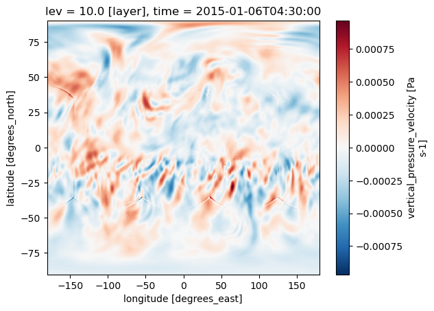
Get the matchups
They with be 3D. OMEGA is vertical velocity. We will get for lev=10 (altitude_index in our dataframe).
CPU times: user 16.3 s, sys: 2.61 s, total: 18.9 s
Wall time: 45 s
| lat | lon | time | altitude_index | OMEGA | |
|---|---|---|---|---|---|
| 0 | -17.432469 | 24.018931 | 2015-08-22 12:00:00 | 10 | 0.000063 |
| 1 | -16.707673 | 14.478041 | 2016-03-24 12:00:00 | 10 | -0.000089 |
| 2 | -83.839933 | 111.134906 | 2015-05-06 12:00:00 | 10 | -0.000008 |
| 3 | 65.250200 | -159.513009 | 2017-10-29 12:00:00 | 10 | 0.000066 |
| 4 | 28.315760 | -1.839657 | 2016-12-14 12:00:00 | 10 | 0.000146 |