ECCO Vrs 4

Estimating the Circulation and Climate of the Ocean (ECCO) uses the MITgcm earth model and "assimilates" millions of real-world observations—including satellite data (altimetry), Argo floats, and ship-based measurements. This creates a 3D reconstruction of the ocean.

Version 4 (1992-2018) is on NASA EarthData. There are many products in ECCO. We will look at 3 products on the 0.5 degree grid.

• ECCO_L4_MIXED_LAYER_DEPTH_05DEG_DAILY_V4R4: mixed layer depth
• ECCO_L4_SSH_05DEG_DAILY_V4R4: sea surface height
• ECCO_L4_TEMP_SALINITY_05DEG_DAILY_V4R4: this has temperature and salinity at depths.

Note: In a virtual machine in AWS us-west-2, where NASA cloud data is, the point matchups are fast. In Colab, say, your compute is not in the same data region nor provider, and the same matchups might take 10x longer.

Prerequisites

The examples here use NASA EarthData and you need to have an account with EarthData. Make sure you can login.

# if needed
!pip install point-collocation cartopy

import earthaccess
earthaccess.login()

<earthaccess.auth.Auth at 0x7fb0cbd1bc20>

Let's see what ECCO collections are available

import earthaccess
results = earthaccess.search_datasets(
    project = 'ECCO',
)
for item in results[0:10]:
    summary = item.summary()
    print(summary["short-name"])

ECCO_L4_ANCILLARY_DATA_V4R4
ECCO_L4_ATM_STATE_05DEG_DAILY_V4R4
ECCO_L4_ATM_STATE_LLC0090GRID_DAILY_V4R4
ECCO_L4_ATM_STATE_05DEG_MONTHLY_V4R4
ECCO_L4_ATM_STATE_LLC0090GRID_MONTHLY_V4R4
ECCO_L4_OCEAN_BOLUS_STREAMFUNCTION_LLC0090GRID_DAILY_V4R4
ECCO_L4_OCEAN_BOLUS_STREAMFUNCTION_LLC0090GRID_MONTHLY_V4R4
ECCO_L4_BOLUS_05DEG_DAILY_V4R4
ECCO_L4_BOLUS_LLC0090GRID_DAILY_V4R4
ECCO_L4_BOLUS_05DEG_MONTHLY_V4R4

Get some sample points over the ocean

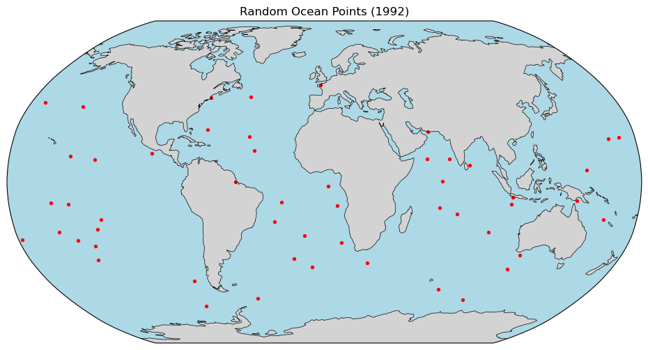
import pandas as pd
url = (
    "https://raw.githubusercontent.com/"
    "fish-pace/point-collocation/main/"
    "examples/fixtures/points_1000.csv"
)
df_points = pd.read_csv(
    url,
    parse_dates=["time"]
)
df = df_points[
    (df_points["time"].dt.year < 2018) &
    (df_points["time"].dt.year > 2014) &
    (df_points["land"] == False)
].reset_index(drop=True)
# Force all timestamps to noon UTC to avoid "midnight overlap" issues
df["time"] = df["time"].dt.normalize() + pd.Timedelta(hours=12)
print(len(df))
df.head()

52

	lat	lon	time	land
0	-2.175441	2.168506	2017-07-02 12:00:00	False
1	-16.216691	76.119033	2015-04-16 12:00:00	False
2	8.500092	82.677680	2015-07-21 12:00:00	False
3	-32.290881	-136.206453	2017-08-09 12:00:00	False
4	-29.495688	-145.182846	2016-02-10 12:00:00	False

Let's plot the points

import matplotlib.pyplot as plt
import cartopy.crs as ccrs
import cartopy.feature as cfeature

# create Robinson projection
proj = ccrs.Robinson()

fig = plt.figure(figsize=(12,6))
ax = plt.axes(projection=proj)

# add map features
ax.add_feature(cfeature.LAND, facecolor="lightgray")
ax.add_feature(cfeature.OCEAN, facecolor="lightblue")
ax.add_feature(cfeature.COASTLINE, linewidth=0.5)

# plot points
ax.scatter(
    df["lon"],
    df["lat"],
    s=8,
    color="red",
    transform=ccrs.PlateCarree()
)

ax.set_global()
plt.title("Random Ocean Points (1992)")
plt.show()

Daily Sea Surface Height

Create the granule plan

import point_collocation as pc
short_name="ECCO_L4_SSH_05DEG_DAILY_V4R4"
plan = pc.plan(
    df,
    data_source="earthaccess",
    source_kwargs={
        "short_name": short_name,
    }
)
plan.summary(n=2)

Plan: 52 points → 52 unique granule(s)
  Points with 0 matches : 0
  Points with >1 matches: 0
  Time buffer: 0 days 00:00:00

First 2 point(s):
  [0] lat=-2.1754, lon=2.1685, time=2017-07-02 12:00:00: 1 match(es)
    → https://archive.podaac.earthdata.nasa.gov/podaac-ops-cumulus-protected/ECCO_L4_SSH_05DEG_DAILY_V4R4/SEA_SURFACE_HEIGHT_day_mean_2017-07-02_ECCO_V4r4_latlon_0p50deg.nc
  [1] lat=-16.2167, lon=76.1190, time=2015-04-16 12:00:00: 1 match(es)
    → https://archive.podaac.earthdata.nasa.gov/podaac-ops-cumulus-protected/ECCO_L4_SSH_05DEG_DAILY_V4R4/SEA_SURFACE_HEIGHT_day_mean_2015-04-16_ECCO_V4r4_latlon_0p50deg.nc

# If needed we can look at the granule metadata
plan.results[0:1]

[Collection: {'Version': 'V4r4', 'ShortName': 'ECCO_L4_SSH_05DEG_DAILY_V4R4'}
 Spatial coverage: {'HorizontalSpatialDomain': {'Geometry': {'BoundingRectangles': [{'WestBoundingCoordinate': -180, 'SouthBoundingCoordinate': -90, 'EastBoundingCoordinate': 180, 'NorthBoundingCoordinate': 90}]}}}
 Temporal coverage: {'RangeDateTime': {'EndingDateTime': '2015-01-12T00:00:00.000Z', 'BeginningDateTime': '2015-01-11T00:00:00.000Z'}}
 Size(MB): 0.9840011596679688
 Data: ['https://archive.podaac.earthdata.nasa.gov/podaac-ops-cumulus-protected/ECCO_L4_SSH_05DEG_DAILY_V4R4/SEA_SURFACE_HEIGHT_day_mean_2015-01-11_ECCO_V4r4_latlon_0p50deg.nc']]

Let's plot a granule to see how it looks

ds = plan.open_dataset(0)
ds

open_method: {'xarray_open': 'dataset', 'open_kwargs': {'chunks': {}, 'engine': 'h5netcdf', 'decode_timedelta': False}, 'coords': 'auto', 'set_coords': True, 'dim_renames': None, 'auto_align_phony_dims': None, 'merge': None}
Geolocation auto detected with cf_xarray: ('longitude', 'latitude') — lon dims=('longitude',), lat dims=('latitude',)

<xarray.Dataset> Size: 3MB
Dimensions:         (time: 1, latitude: 360, longitude: 720, nv: 2)
Coordinates:
  * time            (time) datetime64[ns] 8B 2015-01-11T12:00:00
  * latitude        (latitude) float32 1kB -89.75 -89.25 -88.75 ... 89.25 89.75
  * longitude       (longitude) float32 3kB -179.8 -179.2 -178.8 ... 179.2 179.8
    time_bnds       (time, nv) datetime64[ns] 16B dask.array<chunksize=(1, 2), meta=np.ndarray>
    latitude_bnds   (latitude, nv) float32 3kB dask.array<chunksize=(360, 2), meta=np.ndarray>
    longitude_bnds  (longitude, nv) float32 6kB dask.array<chunksize=(720, 2), meta=np.ndarray>
Dimensions without coordinates: nv
Data variables:
    SSH             (time, latitude, longitude) float32 1MB dask.array<chunksize=(1, 360, 720), meta=np.ndarray>
    SSHIBC          (time, latitude, longitude) float32 1MB dask.array<chunksize=(1, 360, 720), meta=np.ndarray>
    SSHNOIBC        (time, latitude, longitude) float32 1MB dask.array<chunksize=(1, 360, 720), meta=np.ndarray>
Attributes: (12/57)
    acknowledgement:              This research was carried out by the Jet Pr...
    author:                       Ian Fenty and Ou Wang
    cdm_data_type:                Grid
    comment:                      Fields provided on a regular lat-lon grid. ...
    Conventions:                  CF-1.8, ACDD-1.3
    coordinates_comment:          Note: the global 'coordinates' attribute de...
    ...                           ...
    time_coverage_duration:       P1D
    time_coverage_end:            2015-01-12T00:00:00
    time_coverage_resolution:     P1D
    time_coverage_start:          2015-01-11T00:00:00
    title:                        ECCO Sea Surface Height - Daily Mean 0.5 De...
    uuid:                         4f9bf9bc-404a-11eb-93e8-0cc47a3f39b7

xarray.Dataset

• Dimensions:
  • time: 1
  • latitude: 360
  • longitude: 720
  • nv: 2
• Coordinates: (6)
  • time
    (time)
    datetime64[ns]
    2015-01-11T12:00:00

    axis :

    T

    bounds :

    time_bnds

    coverage_content_type :

    coordinate

    long_name :

    center time of averaging period

    standard_name :

    time

    array(['2015-01-11T12:00:00.000000000'], dtype='datetime64[ns]')

  • latitude
    (latitude)
    float32
    -89.75 -89.25 ... 89.25 89.75

    axis :

    Y

    bounds :

    latitude_bnds

    comment :

    uniform grid spacing from -89.75 to 89.75 by 0.5

    coverage_content_type :

    coordinate

    long_name :

    latitude at grid cell center

    standard_name :

    latitude

    units :

    degrees_north

    array([-89.75, -89.25, -88.75, ...,  88.75,  89.25,  89.75],
          shape=(360,), dtype=float32)

  • longitude
    (longitude)
    float32
    -179.8 -179.2 ... 179.2 179.8

    axis :

    X

    bounds :

    longitude_bnds

    comment :

    uniform grid spacing from -179.75 to 179.75 by 0.5

    coverage_content_type :

    coordinate

    long_name :

    longitude at grid cell center

    standard_name :

    longitude

    units :

    degrees_east

    array([-179.75, -179.25, -178.75, ...,  178.75,  179.25,  179.75],
          shape=(720,), dtype=float32)

  • time_bnds
    (time, nv)
    datetime64[ns]
    dask.array<chunksize=(1, 2), meta=np.ndarray>

    comment :

    Start and end times of averaging period.

    coverage_content_type :

    coordinate

    long_name :

    time bounds of averaging period

    Array Chunk Bytes 16 B 16 B Shape (1, 2) (1, 2) Dask graph 1 chunks in 2 graph layers Data type datetime64[ns] numpy.ndarray

  • latitude_bnds
    (latitude, nv)
    float32
    dask.array<chunksize=(360, 2), meta=np.ndarray>

    coverage_content_type :

    coordinate

    long_name :

    latitude bounds grid cells

    Array Chunk Bytes 2.81 kiB 2.81 kiB Shape (360, 2) (360, 2) Dask graph 1 chunks in 2 graph layers Data type float32 numpy.ndarray

  • longitude_bnds
    (longitude, nv)
    float32
    dask.array<chunksize=(720, 2), meta=np.ndarray>

    coverage_content_type :

    coordinate

    long_name :

    longitude bounds grid cells

    Array Chunk Bytes 5.62 kiB 5.62 kiB Shape (720, 2) (720, 2) Dask graph 1 chunks in 2 graph layers Data type float32 numpy.ndarray

• Data variables: (3)
  • SSH
    (time, latitude, longitude)
    float32
    dask.array<chunksize=(1, 360, 720), meta=np.ndarray>

    coverage_content_type :

    modelResult

    long_name :

    Dynamic sea surface height anomaly

    standard_name :

    sea_surface_height_above_geoid

    units :

    m

    comment :

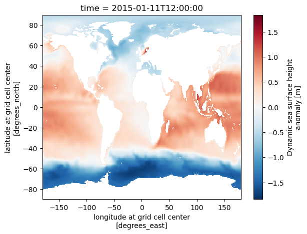
    Dynamic sea surface height anomaly above the geoid, suitable for comparisons with altimetry sea surface height data products that apply the inverse barometer (IB) correction. Note: SSH is calculated by correcting model sea level anomaly ETAN for three effects: a) global mean steric sea level changes related to density changes in the Boussinesq volume-conserving model (Greatbatch correction, see sterGloH), b) the inverted barometer (IB) effect (see SSHIBC) and c) sea level displacement due to sea-ice and snow pressure loading (see sIceLoad). SSH can be compared with the similarly-named SSH variable in previous ECCO products that did not include atmospheric pressure loading (e.g., Version 4 Release 3). Use SSHNOIBC for comparisons with altimetry data products that do NOT apply the IB correction.

    valid_min :

    -2.4861555099487305

    valid_max :

    2.2875382900238037

    Array Chunk Bytes 0.99 MiB 0.99 MiB Shape (1, 360, 720) (1, 360, 720) Dask graph 1 chunks in 2 graph layers Data type float32 numpy.ndarray

  • SSHIBC
    (time, latitude, longitude)
    float32
    dask.array<chunksize=(1, 360, 720), meta=np.ndarray>

    coverage_content_type :

    modelResult

    long_name :

    The inverted barometer (IB) correction to sea surface height due to atmospheric pressure loading

    units :

    m

    comment :

    Not an SSH itself, but a correction to model sea level anomaly (ETAN) required to account for the static part of sea surface displacement by atmosphere pressure loading: SSH = SSHNOIBC - SSHIBC. Note: Use SSH for model-data comparisons with altimetry data products that DO apply the IB correction and SSHNOIBC for comparisons with altimetry data products that do NOT apply the IB correction.

    valid_min :

    -0.5228679180145264

    valid_max :

    0.8955588340759277

    Array Chunk Bytes 0.99 MiB 0.99 MiB Shape (1, 360, 720) (1, 360, 720) Dask graph 1 chunks in 2 graph layers Data type float32 numpy.ndarray

  • SSHNOIBC
    (time, latitude, longitude)
    float32
    dask.array<chunksize=(1, 360, 720), meta=np.ndarray>

    coverage_content_type :

    modelResult

    long_name :

    Sea surface height anomaly without the inverted barometer (IB) correction

    units :

    m

    comment :

    Sea surface height anomaly above the geoid without the inverse barometer (IB) correction, suitable for comparisons with altimetry sea surface height data products that do NOT apply the inverse barometer (IB) correction. Note: SSHNOIBC is calculated by correcting model sea level anomaly ETAN for two effects: a) global mean steric sea level changes related to density changes in the Boussinesq volume-conserving model (Greatbatch correction, see sterGloH), b) sea level displacement due to sea-ice and snow pressure loading (see sIceLoad). In ECCO Version 4 Release 4 the model is forced with atmospheric pressure loading. SSHNOIBC does not correct for the static part of the effect of atmosphere pressure loading on sea surface height (the so-called inverse barometer (IB) correction). Use SSH for comparisons with altimetry data products that DO apply the IB correction.

    valid_min :

    -2.45104718208313

    valid_max :

    2.2390522956848145

    Array Chunk Bytes 0.99 MiB 0.99 MiB Shape (1, 360, 720) (1, 360, 720) Dask graph 1 chunks in 2 graph layers Data type float32 numpy.ndarray

• Attributes: (57)

  acknowledgement :

  This research was carried out by the Jet Propulsion Laboratory, managed by the California Institute of Technology under a contract with the National Aeronautics and Space Administration.

  author :

  Ian Fenty and Ou Wang

  cdm_data_type :

  Grid

  comment :

  Fields provided on a regular lat-lon grid. They have been mapped to the regular lat-lon grid from the original ECCO lat-lon-cap 90 (llc90) native model grid. SSH (dynamic sea surface height) = SSHNOIBC (dynamic sea surface without the inverse barometer correction) - SSHIBC (inverse barometer correction). The inverted barometer correction accounts for variations in sea surface height due to atmospheric pressure variations.

  Conventions :

  CF-1.8, ACDD-1.3

  coordinates_comment :

  Note: the global 'coordinates' attribute describes auxillary coordinates.

  creator_email :

  ecco-group@mit.edu

  creator_institution :

  NASA Jet Propulsion Laboratory (JPL)

  creator_name :

  ECCO Consortium

  creator_type :

  group

  creator_url :

  https://ecco-group.org

  date_created :

  2020-12-17T01:29:07

  date_issued :

  2020-12-17T01:29:07

  date_metadata_modified :

  2021-03-15T23:12:48

  date_modified :

  2021-03-15T23:12:48

  geospatial_bounds_crs :

  EPSG:4326

  geospatial_lat_max :

  90.0

  geospatial_lat_min :

  -90.0

  geospatial_lat_resolution :

  0.5

  geospatial_lat_units :

  degrees_north

  geospatial_lon_max :

  180.0

  geospatial_lon_min :

  -180.0

  geospatial_lon_resolution :

  0.5

  geospatial_lon_units :

  degrees_east

  history :

  Inaugural release of an ECCO Central Estimate solution to PO.DAAC

  id :

  10.5067/ECG5D-SSH44

  institution :

  NASA Jet Propulsion Laboratory (JPL)

  instrument_vocabulary :

  GCMD instrument keywords

  keywords :

  EARTH SCIENCE > OCEANS > SEA SURFACE TOPOGRAPHY > SEA SURFACE HEIGHT, EARTH SCIENCE SERVICES > MODELS > EARTH SCIENCE REANALYSES/ASSIMILATION MODELS

  keywords_vocabulary :

  NASA Global Change Master Directory (GCMD) Science Keywords

  license :

  Public Domain

  metadata_link :

  https://cmr.earthdata.nasa.gov/search/collections.umm_json?ShortName=ECCO_L4_SSH_05DEG_DAILY_V4R4

  naming_authority :

  gov.nasa.jpl

  platform :

  ERS-1/2, TOPEX/Poseidon, Geosat Follow-On (GFO), ENVISAT, Jason-1, Jason-2, CryoSat-2, SARAL/AltiKa, Jason-3, AVHRR, Aquarius, SSM/I, SSMIS, GRACE, DTU17MDT, Argo, WOCE, GO-SHIP, MEOP, Ice Tethered Profilers (ITP)

  platform_vocabulary :

  GCMD platform keywords

  processing_level :

  L4

  product_name :

  SEA_SURFACE_HEIGHT_day_mean_2015-01-11_ECCO_V4r4_latlon_0p50deg.nc

  product_time_coverage_end :

  2018-01-01T00:00:00

  product_time_coverage_start :

  1992-01-01T12:00:00

  product_version :

  Version 4, Release 4

  program :

  NASA Physical Oceanography, Cryosphere, Modeling, Analysis, and Prediction (MAP)

  project :

  Estimating the Circulation and Climate of the Ocean (ECCO)

  publisher_email :

  podaac@podaac.jpl.nasa.gov

  publisher_institution :

  PO.DAAC

  publisher_name :

  Physical Oceanography Distributed Active Archive Center (PO.DAAC)

  publisher_type :

  institution

  publisher_url :

  https://podaac.jpl.nasa.gov

  references :

  ECCO Consortium, Fukumori, I., Wang, O., Fenty, I., Forget, G., Heimbach, P., & Ponte, R. M. 2020. Synopsis of the ECCO Central Production Global Ocean and Sea-Ice State Estimate (Version 4 Release 4). doi:10.5281/zenodo.3765928

  source :

  The ECCO V4r4 state estimate was produced by fitting a free-running solution of the MITgcm (checkpoint 66g) to satellite and in situ observational data in a least squares sense using the adjoint method

  standard_name_vocabulary :

  NetCDF Climate and Forecast (CF) Metadata Convention

  summary :

  This dataset provides daily-averaged dynamic sea surface height interpolated to a regular 0.5-degree grid from the ECCO Version 4 Release 4 (V4r4) ocean and sea-ice state estimate. Estimating the Circulation and Climate of the Ocean (ECCO) state estimates are dynamically and kinematically-consistent reconstructions of the three-dimensional, time-evolving ocean, sea-ice, and surface atmospheric states. ECCO V4r4 is a free-running solution of a global, nominally 1-degree configuration of the MIT general circulation model (MITgcm) that has been fit to observations in a least-squares sense. Observational data constraints used in V4r4 include sea surface height (SSH) from satellite altimeters [ERS-1/2, TOPEX/Poseidon, GFO, ENVISAT, Jason-1,2,3, CryoSat-2, and SARAL/AltiKa]; sea surface temperature (SST) from satellite radiometers [AVHRR], sea surface salinity (SSS) from the Aquarius satellite radiometer/scatterometer, ocean bottom pressure (OBP) from the GRACE satellite gravimeter; sea-ice concentration from satellite radiometers [SSM/I and SSMIS], and in-situ ocean temperature and salinity measured with conductivity-temperature-depth (CTD) sensors and expendable bathythermographs (XBTs) from several programs [e.g., WOCE, GO-SHIP, Argo, and others] and platforms [e.g., research vessels, gliders, moorings, ice-tethered profilers, and instrumented pinnipeds]. V4r4 covers the period 1992-01-01T12:00:00 to 2018-01-01T00:00:00.

  time_coverage_duration :

  P1D

  time_coverage_end :

  2015-01-12T00:00:00

  time_coverage_resolution :

  P1D

  time_coverage_start :

  2015-01-11T00:00:00

  title :

  ECCO Sea Surface Height - Daily Mean 0.5 Degree (Version 4 Release 4)

  uuid :

  4f9bf9bc-404a-11eb-93e8-0cc47a3f39b7

ds.SSH.plot()

<matplotlib.collections.QuadMesh at 0x7f988bade3c0>

Get the matchups

%%time
res = pc.matchup(plan, variables = ["SSH"])

CPU times: user 12.3 s, sys: 97.6 ms, total: 12.4 s
Wall time: 17.5 s

res[['lat', 'lon', 'time', 'SSH']].dropna(subset=['SSH']).head()

	lat	lon	time	SSH
0	-2.175441	2.168506	2017-07-02 12:00:00	0.049727
1	-16.216691	76.119033	2015-04-16 12:00:00	0.795746
2	8.500092	82.677680	2015-07-21 12:00:00	0.555195
3	-32.290881	-136.206453	2017-08-09 12:00:00	0.471952
4	-29.495688	-145.182846	2016-02-10 12:00:00	0.597943

Temperature

Temperature is 3D: lat, lon, depth. We will add depth to our dataframe so we can get temperature at specific depths. Depth is Z in ECCO granules and it is negative. We need to specify the additional coordinate that we are matching, beyond lat, lon, time.

df['depth'] = -1000

coord_spec = {
    "depth": {"source": "Z", "points": "depth"},
}

import point_collocation as pc
short_name="ECCO_L4_TEMP_SALINITY_05DEG_DAILY_V4R4"
plan = pc.plan(
    df,
    data_source="earthaccess",
    source_kwargs={
        "short_name": short_name,
    }
)
plan.summary(n=2)

Plan: 52 points → 52 unique granule(s)
  Points with 0 matches : 0
  Points with >1 matches: 0
  Time buffer: 0 days 00:00:00

First 2 point(s):
  [0] lat=-2.1754, lon=2.1685, time=2017-07-02 12:00:00: 1 match(es)
    → https://archive.podaac.earthdata.nasa.gov/podaac-ops-cumulus-protected/ECCO_L4_TEMP_SALINITY_05DEG_DAILY_V4R4/OCEAN_TEMPERATURE_SALINITY_day_mean_2017-07-02_ECCO_V4r4_latlon_0p50deg.nc
  [1] lat=-16.2167, lon=76.1190, time=2015-04-16 12:00:00: 1 match(es)
    → https://archive.podaac.earthdata.nasa.gov/podaac-ops-cumulus-protected/ECCO_L4_TEMP_SALINITY_05DEG_DAILY_V4R4/OCEAN_TEMPERATURE_SALINITY_day_mean_2015-04-16_ECCO_V4r4_latlon_0p50deg.nc

ds = plan.open_dataset(0)
ds

open_method: {'xarray_open': 'dataset', 'open_kwargs': {'chunks': {}, 'engine': 'h5netcdf', 'decode_timedelta': False}, 'coords': 'auto', 'set_coords': True, 'dim_renames': None, 'auto_align_phony_dims': None, 'merge': None}
Geolocation auto detected with cf_xarray: ('longitude', 'latitude') — lon dims=('longitude',), lat dims=('latitude',); time dim='time' (1 step(s))
Points columns used: y='lat', x='lon', time='time'

<xarray.Dataset> Size: 104MB
Dimensions:         (time: 1, Z: 50, latitude: 360, longitude: 720, nv: 2)
Coordinates:
  * time            (time) datetime64[ns] 8B 2015-01-11T12:00:00
  * Z               (Z) float32 200B -5.0 -15.0 -25.0 ... -5.461e+03 -5.906e+03
  * latitude        (latitude) float32 1kB -89.75 -89.25 -88.75 ... 89.25 89.75
  * longitude       (longitude) float32 3kB -179.8 -179.2 -178.8 ... 179.2 179.8
    time_bnds       (time, nv) datetime64[ns] 16B dask.array<chunksize=(1, 2), meta=np.ndarray>
    latitude_bnds   (latitude, nv) float32 3kB dask.array<chunksize=(360, 2), meta=np.ndarray>
    longitude_bnds  (longitude, nv) float32 6kB dask.array<chunksize=(720, 2), meta=np.ndarray>
    Z_bnds          (Z, nv) float32 400B dask.array<chunksize=(50, 2), meta=np.ndarray>
Dimensions without coordinates: nv
Data variables:
    THETA           (time, Z, latitude, longitude) float32 52MB dask.array<chunksize=(1, 25, 180, 360), meta=np.ndarray>
    SALT            (time, Z, latitude, longitude) float32 52MB dask.array<chunksize=(1, 25, 180, 360), meta=np.ndarray>
Attributes: (12/62)
    acknowledgement:                 This research was carried out by the Jet...
    author:                          Ian Fenty and Ou Wang
    cdm_data_type:                   Grid
    comment:                         Fields provided on a regular lat-lon gri...
    Conventions:                     CF-1.8, ACDD-1.3
    coordinates_comment:             Note: the global 'coordinates' attribute...
    ...                              ...
    time_coverage_duration:          P1D
    time_coverage_end:               2015-01-12T00:00:00
    time_coverage_resolution:        P1D
    time_coverage_start:             2015-01-11T00:00:00
    title:                           ECCO Ocean Temperature and Salinity - Da...
    uuid:                            a8d2856a-412a-11eb-ba7a-0cc47a3f6879

xarray.Dataset

• Dimensions:
  • time: 1
  • Z: 50
  • latitude: 360
  • longitude: 720
  • nv: 2
• Coordinates: (8)
  • time
    (time)
    datetime64[ns]
    2015-01-11T12:00:00

    axis :

    T

    bounds :

    time_bnds

    coverage_content_type :

    coordinate

    long_name :

    center time of averaging period

    standard_name :

    time

    array(['2015-01-11T12:00:00.000000000'], dtype='datetime64[ns]')

  • Z
    (Z)
    float32
    -5.0 -15.0 ... -5.906e+03

    axis :

    Z

    bounds :

    Z_bnds

    comment :

    Non-uniform vertical spacing.

    coverage_content_type :

    coordinate

    long_name :

    depth of grid cell center

    positive :

    up

    standard_name :

    depth

    units :

    m

    array([-5.000000e+00, -1.500000e+01, -2.500000e+01, -3.500000e+01,
           -4.500000e+01, -5.500000e+01, -6.500000e+01, -7.500500e+01,
           -8.502500e+01, -9.509500e+01, -1.053100e+02, -1.158700e+02,
           -1.271500e+02, -1.397400e+02, -1.544700e+02, -1.724000e+02,
           -1.947350e+02, -2.227100e+02, -2.574700e+02, -2.999300e+02,
           -3.506800e+02, -4.099300e+02, -4.774700e+02, -5.527100e+02,
           -6.347350e+02, -7.224000e+02, -8.144700e+02, -9.097400e+02,
           -1.007155e+03, -1.105905e+03, -1.205535e+03, -1.306205e+03,
           -1.409150e+03, -1.517095e+03, -1.634175e+03, -1.765135e+03,
           -1.914150e+03, -2.084035e+03, -2.276225e+03, -2.491250e+03,
           -2.729250e+03, -2.990250e+03, -3.274250e+03, -3.581250e+03,
           -3.911250e+03, -4.264250e+03, -4.640250e+03, -5.039250e+03,
           -5.461250e+03, -5.906250e+03], dtype=float32)

  • latitude
    (latitude)
    float32
    -89.75 -89.25 ... 89.25 89.75

    axis :

    Y

    bounds :

    latitude_bnds

    comment :

    uniform grid spacing from -89.75 to 89.75 by 0.5

    coverage_content_type :

    coordinate

    long_name :

    latitude at grid cell center

    standard_name :

    latitude

    units :

    degrees_north

    array([-89.75, -89.25, -88.75, ...,  88.75,  89.25,  89.75],
          shape=(360,), dtype=float32)

  • longitude
    (longitude)
    float32
    -179.8 -179.2 ... 179.2 179.8

    axis :

    X

    bounds :

    longitude_bnds

    comment :

    uniform grid spacing from -179.75 to 179.75 by 0.5

    coverage_content_type :

    coordinate

    long_name :

    longitude at grid cell center

    standard_name :

    longitude

    units :

    degrees_east

    array([-179.75, -179.25, -178.75, ...,  178.75,  179.25,  179.75],
          shape=(720,), dtype=float32)

  • time_bnds
    (time, nv)
    datetime64[ns]
    dask.array<chunksize=(1, 2), meta=np.ndarray>

    comment :

    Start and end times of averaging period.

    coverage_content_type :

    coordinate

    long_name :

    time bounds of averaging period

    Array Chunk Bytes 16 B 16 B Shape (1, 2) (1, 2) Dask graph 1 chunks in 2 graph layers Data type datetime64[ns] numpy.ndarray

  • latitude_bnds
    (latitude, nv)
    float32
    dask.array<chunksize=(360, 2), meta=np.ndarray>

    coverage_content_type :

    coordinate

    long_name :

    latitude bounds grid cells

    Array Chunk Bytes 2.81 kiB 2.81 kiB Shape (360, 2) (360, 2) Dask graph 1 chunks in 2 graph layers Data type float32 numpy.ndarray

  • longitude_bnds
    (longitude, nv)
    float32
    dask.array<chunksize=(720, 2), meta=np.ndarray>

    coverage_content_type :

    coordinate

    long_name :

    longitude bounds grid cells

    Array Chunk Bytes 5.62 kiB 5.62 kiB Shape (720, 2) (720, 2) Dask graph 1 chunks in 2 graph layers Data type float32 numpy.ndarray

  • Z_bnds
    (Z, nv)
    float32
    dask.array<chunksize=(50, 2), meta=np.ndarray>

    comment :

    One pair of bounds for each vertical level.

    coverage_content_type :

    coordinate

    long_name :

    depths of grid cell upper and lower interfaces

    Array Chunk Bytes 400 B 400 B Shape (50, 2) (50, 2) Dask graph 1 chunks in 2 graph layers Data type float32 numpy.ndarray

• Data variables: (2)
  • THETA
    (time, Z, latitude, longitude)
    float32
    dask.array<chunksize=(1, 25, 180, 360), meta=np.ndarray>

    coverage_content_type :

    modelResult

    long_name :

    Potential temperature

    standard_name :

    sea_water_potential_temperature

    units :

    degree_C

    comment :

    Sea water potential temperature is the temperature a parcel of sea water would have if moved adiabatically to sea level pressure. Note: the equation of state is a modified UNESCO formula by Jackett and McDougall (1995), which uses the model variable potential temperature as input assuming a horizontally and temporally constant pressure of $p_0=-g ho_{0} z$.

    valid_min :

    -2.9179372787475586

    valid_max :

    36.425140380859375

    Array Chunk Bytes 49.44 MiB 6.18 MiB Shape (1, 50, 360, 720) (1, 25, 180, 360) Dask graph 8 chunks in 2 graph layers Data type float32 numpy.ndarray

  • SALT
    (time, Z, latitude, longitude)
    float32
    dask.array<chunksize=(1, 25, 180, 360), meta=np.ndarray>

    coverage_content_type :

    modelResult

    long_name :

    Salinity

    standard_name :

    sea_water_salinity

    units :

    1e-3

    valid_min :

    16.73577880859375

    valid_max :

    41.321231842041016

    comment :

    Defined using CF convention 'Sea water salinity is the salt content of sea water, often on the Practical Salinity Scale of 1978. However, the unqualified term 'salinity' is generic and does not necessarily imply any particular method of calculation. The units of salinity are dimensionless and the units attribute should normally be given as 1e-3 or 0.001 i.e. parts per thousand.' see https://cfconventions.org/Data/cf-standard-names/73/build/cf-standard-name-table.html

    Array Chunk Bytes 49.44 MiB 6.18 MiB Shape (1, 50, 360, 720) (1, 25, 180, 360) Dask graph 8 chunks in 2 graph layers Data type float32 numpy.ndarray

• Attributes: (62)

  acknowledgement :

  This research was carried out by the Jet Propulsion Laboratory, managed by the California Institute of Technology under a contract with the National Aeronautics and Space Administration.

  author :

  Ian Fenty and Ou Wang

  cdm_data_type :

  Grid

  comment :

  Fields provided on a regular lat-lon grid. They have been mapped to the regular lat-lon grid from the original ECCO lat-lon-cap 90 (llc90) native model grid.

  Conventions :

  CF-1.8, ACDD-1.3

  coordinates_comment :

  Note: the global 'coordinates' attribute describes auxillary coordinates.

  creator_email :

  ecco-group@mit.edu

  creator_institution :

  NASA Jet Propulsion Laboratory (JPL)

  creator_name :

  ECCO Consortium

  creator_type :

  group

  creator_url :

  https://ecco-group.org

  date_created :

  2020-12-18T04:15:04

  date_issued :

  2020-12-18T04:15:04

  date_metadata_modified :

  2021-03-15T23:53:01

  date_modified :

  2021-03-15T23:53:01

  geospatial_bounds_crs :

  EPSG:4326

  geospatial_lat_max :

  90.0

  geospatial_lat_min :

  -90.0

  geospatial_lat_resolution :

  0.5

  geospatial_lat_units :

  degrees_north

  geospatial_lon_max :

  180.0

  geospatial_lon_min :

  -180.0

  geospatial_lon_resolution :

  0.5

  geospatial_lon_units :

  degrees_east

  geospatial_vertical_max :

  0.0

  geospatial_vertical_min :

  -6134.5

  geospatial_vertical_positive :

  up

  geospatial_vertical_resolution :

  variable

  geospatial_vertical_units :

  meter

  history :

  Inaugural release of an ECCO Central Estimate solution to PO.DAAC

  id :

  10.5067/ECG5D-OTS44

  institution :

  NASA Jet Propulsion Laboratory (JPL)

  instrument_vocabulary :

  GCMD instrument keywords

  keywords :

  EARTH SCIENCE > OCEANS > OCEAN TEMPERATURE > POTENTIAL TEMPERATURE, EARTH SCIENCE > OCEANS > SALINITY/DENSITY > SALINITY, EARTH SCIENCE SERVICES > MODELS > EARTH SCIENCE REANALYSES/ASSIMILATION MODELS

  keywords_vocabulary :

  NASA Global Change Master Directory (GCMD) Science Keywords

  license :

  Public Domain

  metadata_link :

  https://cmr.earthdata.nasa.gov/search/collections.umm_json?ShortName=ECCO_L4_TEMP_SALINITY_05DEG_DAILY_V4R4

  naming_authority :

  gov.nasa.jpl

  platform :

  ERS-1/2, TOPEX/Poseidon, Geosat Follow-On (GFO), ENVISAT, Jason-1, Jason-2, CryoSat-2, SARAL/AltiKa, Jason-3, AVHRR, Aquarius, SSM/I, SSMIS, GRACE, DTU17MDT, Argo, WOCE, GO-SHIP, MEOP, Ice Tethered Profilers (ITP)

  platform_vocabulary :

  GCMD platform keywords

  processing_level :

  L4

  product_name :

  OCEAN_TEMPERATURE_SALINITY_day_mean_2015-01-11_ECCO_V4r4_latlon_0p50deg.nc

  product_time_coverage_end :

  2018-01-01T00:00:00

  product_time_coverage_start :

  1992-01-01T12:00:00

  product_version :

  Version 4, Release 4

  program :

  NASA Physical Oceanography, Cryosphere, Modeling, Analysis, and Prediction (MAP)

  project :

  Estimating the Circulation and Climate of the Ocean (ECCO)

  publisher_email :

  podaac@podaac.jpl.nasa.gov

  publisher_institution :

  PO.DAAC

  publisher_name :

  Physical Oceanography Distributed Active Archive Center (PO.DAAC)

  publisher_type :

  institution

  publisher_url :

  https://podaac.jpl.nasa.gov

  references :

  ECCO Consortium, Fukumori, I., Wang, O., Fenty, I., Forget, G., Heimbach, P., & Ponte, R. M. 2020. Synopsis of the ECCO Central Production Global Ocean and Sea-Ice State Estimate (Version 4 Release 4). doi:10.5281/zenodo.3765928

  source :

  The ECCO V4r4 state estimate was produced by fitting a free-running solution of the MITgcm (checkpoint 66g) to satellite and in situ observational data in a least squares sense using the adjoint method

  standard_name_vocabulary :

  NetCDF Climate and Forecast (CF) Metadata Convention

  summary :

  This dataset provides daily-averaged ocean potential temperature and salinity interpolated to a regular 0.5-degree grid from the ECCO Version 4 Release 4 (V4r4) ocean and sea-ice state estimate. Estimating the Circulation and Climate of the Ocean (ECCO) state estimates are dynamically and kinematically-consistent reconstructions of the three-dimensional, time-evolving ocean, sea-ice, and surface atmospheric states. ECCO V4r4 is a free-running solution of a global, nominally 1-degree configuration of the MIT general circulation model (MITgcm) that has been fit to observations in a least-squares sense. Observational data constraints used in V4r4 include sea surface height (SSH) from satellite altimeters [ERS-1/2, TOPEX/Poseidon, GFO, ENVISAT, Jason-1,2,3, CryoSat-2, and SARAL/AltiKa]; sea surface temperature (SST) from satellite radiometers [AVHRR], sea surface salinity (SSS) from the Aquarius satellite radiometer/scatterometer, ocean bottom pressure (OBP) from the GRACE satellite gravimeter; sea-ice concentration from satellite radiometers [SSM/I and SSMIS], and in-situ ocean temperature and salinity measured with conductivity-temperature-depth (CTD) sensors and expendable bathythermographs (XBTs) from several programs [e.g., WOCE, GO-SHIP, Argo, and others] and platforms [e.g., research vessels, gliders, moorings, ice-tethered profilers, and instrumented pinnipeds]. V4r4 covers the period 1992-01-01T12:00:00 to 2018-01-01T00:00:00.

  time_coverage_duration :

  P1D

  time_coverage_end :

  2015-01-12T00:00:00

  time_coverage_resolution :

  P1D

  time_coverage_start :

  2015-01-11T00:00:00

  title :

  ECCO Ocean Temperature and Salinity - Daily Mean 0.5 Degree (Version 4 Release 4)

  uuid :

  a8d2856a-412a-11eb-ba7a-0cc47a3f6879

Get the matchups for potential temperature

They with be 3D. Variable at 50 depths. THETA is temperature at -1000 meters, which is the depth value in our dataframe.

%%time
res = pc.matchup(plan, variables = ["THETA"], coord_spec=coord_spec)

CPU times: user 16.4 s, sys: 1.3 s, total: 17.7 s
Wall time: 44 s

res[['lat', 'lon', 'time', 'depth', 'THETA']].head()

	lat	lon	time	depth	THETA
0	-2.175441	2.168506	2017-07-02 12:00:00	-1000	4.333574
1	-16.216691	76.119033	2015-04-16 12:00:00	-1000	5.358678
2	8.500092	82.677680	2015-07-21 12:00:00	-1000	6.668801
3	-32.290881	-136.206453	2017-08-09 12:00:00	-1000	4.466073
4	-29.495688	-145.182846	2016-02-10 12:00:00	-1000	4.450537

Mixed Layer Depth

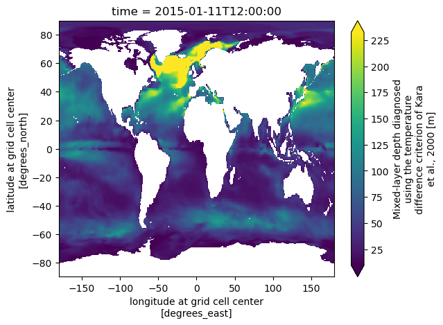
Mixed Layer Depth (MLD) is the thickness of the uppermost layer of the ocean where the water properties (temperature, salinity, and density) are nearly uniform with depth and mixed by wind. Below the MLD is the thermocline, between the MLD and roughly 1,000m, the temperature rapidly drops and density increases. Below the thermocline is the deep ocean, which is cold and dense.

import point_collocation as pc
short_name="ECCO_L4_MIXED_LAYER_DEPTH_05DEG_DAILY_V4R4"
plan = pc.plan(
    df,
    data_source="earthaccess",
    source_kwargs={
        "short_name": short_name,
    }
)
plan.summary(n=2)

Plan: 52 points → 52 unique granule(s)
  Points with 0 matches : 0
  Points with >1 matches: 0
  Time buffer: 0 days 00:00:00

First 2 point(s):
  [0] lat=-2.1754, lon=2.1685, time=2017-07-02 12:00:00: 1 match(es)
    → https://archive.podaac.earthdata.nasa.gov/podaac-ops-cumulus-protected/ECCO_L4_MIXED_LAYER_DEPTH_05DEG_DAILY_V4R4/OCEAN_MIXED_LAYER_DEPTH_day_mean_2017-07-02_ECCO_V4r4_latlon_0p50deg.nc
  [1] lat=-16.2167, lon=76.1190, time=2015-04-16 12:00:00: 1 match(es)
    → https://archive.podaac.earthdata.nasa.gov/podaac-ops-cumulus-protected/ECCO_L4_MIXED_LAYER_DEPTH_05DEG_DAILY_V4R4/OCEAN_MIXED_LAYER_DEPTH_day_mean_2015-04-16_ECCO_V4r4_latlon_0p50deg.nc

ds = plan.open_dataset(0)
ds

open_method: {'xarray_open': 'dataset', 'open_kwargs': {'chunks': {}, 'engine': 'h5netcdf', 'decode_timedelta': False}, 'coords': 'auto', 'set_coords': True, 'dim_renames': None, 'auto_align_phony_dims': None, 'merge': None}
Geolocation auto detected with cf_xarray: ('longitude', 'latitude') — lon dims=('longitude',), lat dims=('latitude',)

<xarray.Dataset> Size: 1MB
Dimensions:         (time: 1, latitude: 360, longitude: 720, nv: 2)
Coordinates:
  * time            (time) datetime64[ns] 8B 2015-01-11T12:00:00
  * latitude        (latitude) float32 1kB -89.75 -89.25 -88.75 ... 89.25 89.75
  * longitude       (longitude) float32 3kB -179.8 -179.2 -178.8 ... 179.2 179.8
    time_bnds       (time, nv) datetime64[ns] 16B dask.array<chunksize=(1, 2), meta=np.ndarray>
    latitude_bnds   (latitude, nv) float32 3kB dask.array<chunksize=(360, 2), meta=np.ndarray>
    longitude_bnds  (longitude, nv) float32 6kB dask.array<chunksize=(720, 2), meta=np.ndarray>
Dimensions without coordinates: nv
Data variables:
    MXLDEPTH        (time, latitude, longitude) float32 1MB dask.array<chunksize=(1, 360, 720), meta=np.ndarray>
Attributes: (12/57)
    acknowledgement:              This research was carried out by the Jet Pr...
    author:                       Ian Fenty and Ou Wang
    cdm_data_type:                Grid
    comment:                      Fields provided on a regular lat-lon grid. ...
    Conventions:                  CF-1.8, ACDD-1.3
    coordinates_comment:          Note: the global 'coordinates' attribute de...
    ...                           ...
    time_coverage_duration:       P1D
    time_coverage_end:            2015-01-12T00:00:00
    time_coverage_resolution:     P1D
    time_coverage_start:          2015-01-11T00:00:00
    title:                        ECCO Ocean Mixed Layer Depth - Daily Mean 0...
    uuid:                         7ce9f68c-4052-11eb-bc70-0cc47a3f3a7f

xarray.Dataset

• Dimensions:
  • time: 1
  • latitude: 360
  • longitude: 720
  • nv: 2
• Coordinates: (6)
  • time
    (time)
    datetime64[ns]
    2015-01-11T12:00:00

    axis :

    T

    bounds :

    time_bnds

    coverage_content_type :

    coordinate

    long_name :

    center time of averaging period

    standard_name :

    time

    array(['2015-01-11T12:00:00.000000000'], dtype='datetime64[ns]')

  • latitude
    (latitude)
    float32
    -89.75 -89.25 ... 89.25 89.75

    axis :

    Y

    bounds :

    latitude_bnds

    comment :

    uniform grid spacing from -89.75 to 89.75 by 0.5

    coverage_content_type :

    coordinate

    long_name :

    latitude at grid cell center

    standard_name :

    latitude

    units :

    degrees_north

    array([-89.75, -89.25, -88.75, ...,  88.75,  89.25,  89.75],
          shape=(360,), dtype=float32)

  • longitude
    (longitude)
    float32
    -179.8 -179.2 ... 179.2 179.8

    axis :

    X

    bounds :

    longitude_bnds

    comment :

    uniform grid spacing from -179.75 to 179.75 by 0.5

    coverage_content_type :

    coordinate

    long_name :

    longitude at grid cell center

    standard_name :

    longitude

    units :

    degrees_east

    array([-179.75, -179.25, -178.75, ...,  178.75,  179.25,  179.75],
          shape=(720,), dtype=float32)

  • time_bnds
    (time, nv)
    datetime64[ns]
    dask.array<chunksize=(1, 2), meta=np.ndarray>

    comment :

    Start and end times of averaging period.

    coverage_content_type :

    coordinate

    long_name :

    time bounds of averaging period

    Array Chunk Bytes 16 B 16 B Shape (1, 2) (1, 2) Dask graph 1 chunks in 2 graph layers Data type datetime64[ns] numpy.ndarray

  • latitude_bnds
    (latitude, nv)
    float32
    dask.array<chunksize=(360, 2), meta=np.ndarray>

    coverage_content_type :

    coordinate

    long_name :

    latitude bounds grid cells

    Array Chunk Bytes 2.81 kiB 2.81 kiB Shape (360, 2) (360, 2) Dask graph 1 chunks in 2 graph layers Data type float32 numpy.ndarray

  • longitude_bnds
    (longitude, nv)
    float32
    dask.array<chunksize=(720, 2), meta=np.ndarray>

    coverage_content_type :

    coordinate

    long_name :

    longitude bounds grid cells

    Array Chunk Bytes 5.62 kiB 5.62 kiB Shape (720, 2) (720, 2) Dask graph 1 chunks in 2 graph layers Data type float32 numpy.ndarray

• Data variables: (1)
  • MXLDEPTH
    (time, latitude, longitude)
    float32
    dask.array<chunksize=(1, 360, 720), meta=np.ndarray>

    coverage_content_type :

    modelResult

    long_name :

    Mixed-layer depth diagnosed using the temperature difference criterion of Kara et al., 2000

    standard_name :

    ocean_mixed_layer_thickness

    units :

    m

    comment :

    Mixed-layer depth as determined by the depth where waters are first 0.8 degrees Celsius colder than the surface. See Kara et al. (JGR, 2000). . Note: the Kara et al. criterion may not be appropriate for some applications. If needed, mixed layer depth can be calculated using different criteria. See vertical density stratification (DRHODR) and density anomaly (RHOAnoma).

    valid_min :

    5.000001430511475

    valid_max :

    5331.2001953125

    Array Chunk Bytes 0.99 MiB 0.99 MiB Shape (1, 360, 720) (1, 360, 720) Dask graph 1 chunks in 2 graph layers Data type float32 numpy.ndarray

• Attributes: (57)

  acknowledgement :

  This research was carried out by the Jet Propulsion Laboratory, managed by the California Institute of Technology under a contract with the National Aeronautics and Space Administration.

  author :

  Ian Fenty and Ou Wang

  cdm_data_type :

  Grid

  comment :

  Fields provided on a regular lat-lon grid. They have been mapped to the regular lat-lon grid from the original ECCO lat-lon-cap 90 (llc90) native model grid.

  Conventions :

  CF-1.8, ACDD-1.3

  coordinates_comment :

  Note: the global 'coordinates' attribute describes auxillary coordinates.

  creator_email :

  ecco-group@mit.edu

  creator_institution :

  NASA Jet Propulsion Laboratory (JPL)

  creator_name :

  ECCO Consortium

  creator_type :

  group

  creator_url :

  https://ecco-group.org

  date_created :

  2020-12-17T02:27:39

  date_issued :

  2020-12-17T02:27:39

  date_metadata_modified :

  2021-03-15T23:05:46

  date_modified :

  2021-03-15T23:05:46

  geospatial_bounds_crs :

  EPSG:4326

  geospatial_lat_max :

  90.0

  geospatial_lat_min :

  -90.0

  geospatial_lat_resolution :

  0.5

  geospatial_lat_units :

  degrees_north

  geospatial_lon_max :

  180.0

  geospatial_lon_min :

  -180.0

  geospatial_lon_resolution :

  0.5

  geospatial_lon_units :

  degrees_east

  history :

  Inaugural release of an ECCO Central Estimate solution to PO.DAAC

  id :

  10.5067/ECG5D-OML44

  institution :

  NASA Jet Propulsion Laboratory (JPL)

  instrument_vocabulary :

  GCMD instrument keywords

  keywords :

  EARTH SCIENCE > OCEANS > OCEAN CIRCULATION > OCEAN MIXED LAYER, EARTH SCIENCE SERVICES > MODELS > EARTH SCIENCE REANALYSES/ASSIMILATION MODELS

  keywords_vocabulary :

  NASA Global Change Master Directory (GCMD) Science Keywords

  license :

  Public Domain

  metadata_link :

  https://cmr.earthdata.nasa.gov/search/collections.umm_json?ShortName=ECCO_L4_MIXED_LAYER_DEPTH_05DEG_DAILY_V4R4

  naming_authority :

  gov.nasa.jpl

  platform :

  ERS-1/2, TOPEX/Poseidon, Geosat Follow-On (GFO), ENVISAT, Jason-1, Jason-2, CryoSat-2, SARAL/AltiKa, Jason-3, AVHRR, Aquarius, SSM/I, SSMIS, GRACE, DTU17MDT, Argo, WOCE, GO-SHIP, MEOP, Ice Tethered Profilers (ITP)

  platform_vocabulary :

  GCMD platform keywords

  processing_level :

  L4

  product_name :

  OCEAN_MIXED_LAYER_DEPTH_day_mean_2015-01-11_ECCO_V4r4_latlon_0p50deg.nc

  product_time_coverage_end :

  2018-01-01T00:00:00

  product_time_coverage_start :

  1992-01-01T12:00:00

  product_version :

  Version 4, Release 4

  program :

  NASA Physical Oceanography, Cryosphere, Modeling, Analysis, and Prediction (MAP)

  project :

  Estimating the Circulation and Climate of the Ocean (ECCO)

  publisher_email :

  podaac@podaac.jpl.nasa.gov

  publisher_institution :

  PO.DAAC

  publisher_name :

  Physical Oceanography Distributed Active Archive Center (PO.DAAC)

  publisher_type :

  institution

  publisher_url :

  https://podaac.jpl.nasa.gov

  references :

  ECCO Consortium, Fukumori, I., Wang, O., Fenty, I., Forget, G., Heimbach, P., & Ponte, R. M. 2020. Synopsis of the ECCO Central Production Global Ocean and Sea-Ice State Estimate (Version 4 Release 4). doi:10.5281/zenodo.3765928

  source :

  The ECCO V4r4 state estimate was produced by fitting a free-running solution of the MITgcm (checkpoint 66g) to satellite and in situ observational data in a least squares sense using the adjoint method

  standard_name_vocabulary :

  NetCDF Climate and Forecast (CF) Metadata Convention

  summary :

  This dataset provides daily-averaged ocean mixed layer depth interpolated to a regular 0.5-degree grid from the ECCO Version 4 Release 4 (V4r4) ocean and sea-ice state estimate. Estimating the Circulation and Climate of the Ocean (ECCO) state estimates are dynamically and kinematically-consistent reconstructions of the three-dimensional, time-evolving ocean, sea-ice, and surface atmospheric states. ECCO V4r4 is a free-running solution of a global, nominally 1-degree configuration of the MIT general circulation model (MITgcm) that has been fit to observations in a least-squares sense. Observational data constraints used in V4r4 include sea surface height (SSH) from satellite altimeters [ERS-1/2, TOPEX/Poseidon, GFO, ENVISAT, Jason-1,2,3, CryoSat-2, and SARAL/AltiKa]; sea surface temperature (SST) from satellite radiometers [AVHRR], sea surface salinity (SSS) from the Aquarius satellite radiometer/scatterometer, ocean bottom pressure (OBP) from the GRACE satellite gravimeter; sea-ice concentration from satellite radiometers [SSM/I and SSMIS], and in-situ ocean temperature and salinity measured with conductivity-temperature-depth (CTD) sensors and expendable bathythermographs (XBTs) from several programs [e.g., WOCE, GO-SHIP, Argo, and others] and platforms [e.g., research vessels, gliders, moorings, ice-tethered profilers, and instrumented pinnipeds]. V4r4 covers the period 1992-01-01T12:00:00 to 2018-01-01T00:00:00.

  time_coverage_duration :

  P1D

  time_coverage_end :

  2015-01-12T00:00:00

  time_coverage_resolution :

  P1D

  time_coverage_start :

  2015-01-11T00:00:00

  title :

  ECCO Ocean Mixed Layer Depth - Daily Mean 0.5 Degree (Version 4 Release 4)

  uuid :

  7ce9f68c-4052-11eb-bc70-0cc47a3f3a7f

ds.MXLDEPTH.plot(robust=True)

<matplotlib.collections.QuadMesh at 0x7f2a83d2e120>

Get matchups

%%time
res = pc.matchup(plan, variables = ["MXLDEPTH"])

CPU times: user 11.7 s, sys: 73.8 ms, total: 11.8 s
Wall time: 17.3 s

res[['lat', 'lon', 'time', 'MXLDEPTH']].dropna(subset=['MXLDEPTH']).head()

	lat	lon	time	MXLDEPTH
0	-2.175441	2.168506	2017-07-02 12:00:00	18.219427
1	-16.216691	76.119033	2015-04-16 12:00:00	38.249325
2	8.500092	82.677680	2015-07-21 12:00:00	38.327206
3	-32.290881	-136.206453	2017-08-09 12:00:00	117.164932
4	-29.495688	-145.182846	2016-02-10 12:00:00	21.410013