MUR SST L4
The Multi-scale Ultra-high Resolution (MUR) Sea Surface Temperature (SST) Level-4 products provide gap-free, globally gridded analyses by combining multiple satellite and in situ observations using interpolation and data fusion techniques. We will compare 2 MUR products. Both are on a regular grid:
MUR-JPL-L4-GLOB-v4.1 (~1 km resolution) High-resolution SST ~2002–present
MUR25-JPL-L4-GLOB-v04.2 (~25 km resolution) Coarse global SST analysis ~1992–2017 (retrospective)
Note: In a virtual machine in AWS us-west-2, where NASA cloud data is, the point matchups are fast. In Colab, say, your compute is not in the same data region nor provider, and the same matchups might take 10x longer.
Prerequisites
The examples here use NASA EarthData and you need to have an account with EarthData. Make sure you can login.
# if needed
! pip install point - collocation cartopy
import earthaccess
earthaccess . login ()
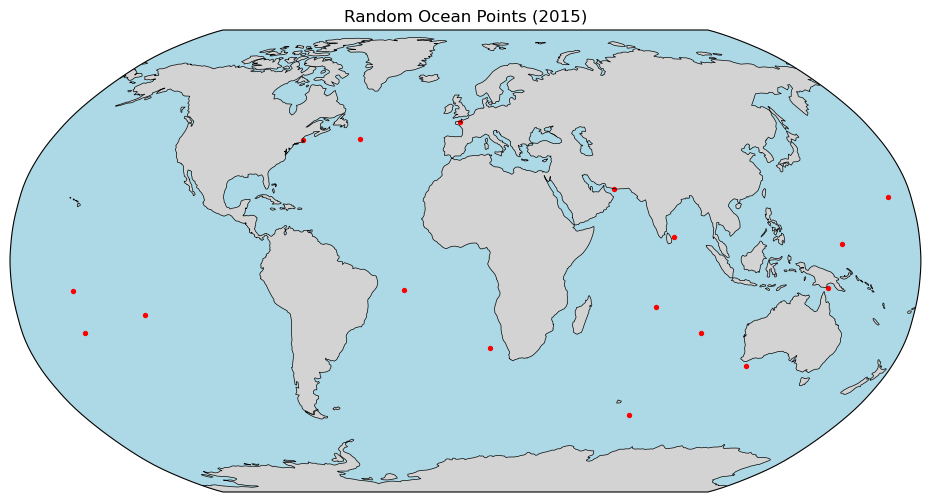
Create some points
Random global over ocean.
import pandas as pd
url = (
"https://raw.githubusercontent.com/"
"fish-pace/point-collocation/main/"
"examples/fixtures/points_1000.csv"
)
df_points = pd . read_csv (
url ,
parse_dates = [ "time" ]
)
df = df_points [
( df_points [ "time" ] . dt . year == 2015 ) &
( df_points [ "land" ] == False )
]
print ( len ( df ))
df . head ()
lat
lon
time
land
45
-16.216691
76.119033
2015-04-16
False
52
8.500092
82.677680
2015-07-21
False
251
5.963712
149.291272
2015-02-07
False
377
-10.447214
-155.929463
2015-10-30
False
384
-30.208351
10.304799
2015-01-12
False
import matplotlib.pyplot as plt
import cartopy.crs as ccrs
import cartopy.feature as cfeature
# create Robinson projection
proj = ccrs . Robinson ()
fig = plt . figure ( figsize = ( 12 , 6 ))
ax = plt . axes ( projection = proj )
# add map features
ax . add_feature ( cfeature . LAND , facecolor = "lightgray" )
ax . add_feature ( cfeature . OCEAN , facecolor = "lightblue" )
ax . add_feature ( cfeature . COASTLINE , linewidth = 0.5 )
# plot points
ax . scatter (
df [ "lon" ],
df [ "lat" ],
s = 8 ,
color = "red" ,
transform = ccrs . PlateCarree ()
)
ax . set_global ()
plt . title ( "Random Ocean Points (2015)" )
plt . show ()
Make a plan
import point_collocation as pc
short_name = "MUR-JPL-L4-GLOB-v4.1"
plan = pc . plan (
df ,
data_source = "earthaccess" ,
source_kwargs = {
"short_name" : short_name ,
}
)
plan . summary ( n = 1 )
Plan: 17 points → 17 unique granule(s)
  Points with 0 matches : 0
  Points with >1 matches: 0
  Time buffer: 0 days 00:00:00

First 1 point(s):
  [45] lat=-16.2167, lon=76.1190, time=2015-04-16 00:00:00: 1 match(es)
    → https://archive.podaac.earthdata.nasa.gov/podaac-ops-cumulus-protected/MUR-JPL-L4-GLOB-v4.1/20150416090000-JPL-L4_GHRSST-SSTfnd-MUR-GLOB-v02.0-fv04.1.nc
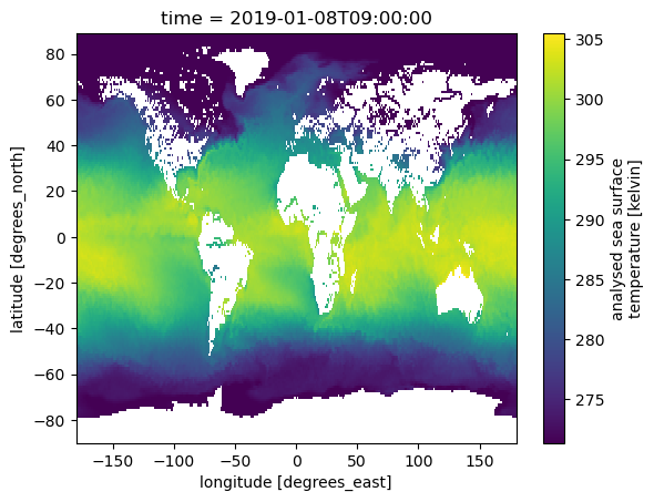
Check out the data first
Hmm, very high resolution.
ds = plan . open_dataset ( 0 )
ds
open_method: {'xarray_open': 'dataset', 'open_kwargs': {'chunks': {}, 'engine': 'h5netcdf', 'decode_timedelta': False}, 'coords': 'auto', 'set_coords': True, 'dim_renames': None, 'auto_align_phony_dims': None, 'merge': None}
Geolocation auto detected with cf_xarray: ('lon', 'lat') — lon dims=('lon',), lat dims=('lat',)
<xarray.Dataset> Size: 21GB
Dimensions:           (time: 1, lat: 17999, lon: 36000)
Coordinates:
  * time              (time) datetime64[ns] 8B 2015-01-12T09:00:00
  * lat               (lat) float32 72kB -89.99 -89.98 -89.97 ... 89.98 89.99
  * lon               (lon) float32 144kB -180.0 -180.0 -180.0 ... 180.0 180.0
Data variables:
    analysed_sst      (time, lat, lon) float64 5GB dask.array<chunksize=(1, 1023, 2047), meta=np.ndarray>
    analysis_error    (time, lat, lon) float64 5GB dask.array<chunksize=(1, 1023, 2047), meta=np.ndarray>
    mask              (time, lat, lon) float32 3GB dask.array<chunksize=(1, 1447, 2895), meta=np.ndarray>
    sea_ice_fraction  (time, lat, lon) float64 5GB dask.array<chunksize=(1, 1447, 2895), meta=np.ndarray>
    dt_1km_data       (time, lat, lon) float32 3GB dask.array<chunksize=(1, 1447, 2895), meta=np.ndarray>
Attributes: (12/47)
    Conventions:                CF-1.5
    title:                      Daily MUR SST, Final product
    summary:                    A merged, multi-sensor L4 Foundation SST anal...
    references:                 http://podaac.jpl.nasa.gov/Multi-scale_Ultra-...
    institution:                Jet Propulsion Laboratory
    history:                    created at nominal 4-day latency; replaced nr...
    ...                         ...
    project:                    NASA Making Earth Science Data Records for Us...
    publisher_name:             GHRSST Project Office
    publisher_url:              http://www.ghrsst.org
    publisher_email:            ghrsst-po@nceo.ac.uk
    processing_level:           L4
cdm_data_type: grid Dimensions: time : 1lat : 17999lon : 36000
Coordinates: (3)
Data variables: (5)
analysed_sst
(time, lat, lon)
float64
dask.array<chunksize=(1, 1023, 2047), meta=np.ndarray>
long_name : analysed sea surface temperature standard_name : sea_surface_foundation_temperature units : kelvin valid_min : -32767 valid_max : 32767 comment : "Final" version using Multi-Resolution Variational Analysis (MRVA) method for interpolation source : AVHRR19_G-NAVO, AVHRR_METOP_A-EUMETSAT, MODIS_A-JPL, MODIS_T-JPL, WSAT-REMSS, iQUAM-NOAA/NESDIS, Ice_Conc-OSISAF
Array
Chunk
Bytes
4.83 GiB
15.98 MiB
Shape
(1, 17999, 36000)
(1, 1023, 2047)
Dask graph
324 chunks in 2 graph layers
Data type
float64 numpy.ndarray
36000
17999
1
analysis_error
(time, lat, lon)
float64
dask.array<chunksize=(1, 1023, 2047), meta=np.ndarray>
long_name : estimated error standard deviation of analysed_sst units : kelvin valid_min : 0 valid_max : 32767 comment : none
Array
Chunk
Bytes
4.83 GiB
15.98 MiB
Shape
(1, 17999, 36000)
(1, 1023, 2047)
Dask graph
324 chunks in 2 graph layers
Data type
float64 numpy.ndarray
36000
17999
1
mask
(time, lat, lon)
float32
dask.array<chunksize=(1, 1447, 2895), meta=np.ndarray>
long_name : sea/land field composite mask valid_min : 1 valid_max : 31 flag_masks : [ 1 2 4 8 16] flag_values : [ 1 2 5 9 13] flag_meanings : 1=open-sea, 2=land, 5=open-lake, 9=open-sea with ice in the grid, 13=open-lake with ice in the grid comment : mask can be used to further filter the data. source : GMT "grdlandmask", ice flag from sea_ice_fraction data
Array
Chunk
Bytes
2.41 GiB
15.98 MiB
Shape
(1, 17999, 36000)
(1, 1447, 2895)
Dask graph
169 chunks in 2 graph layers
Data type
float32 numpy.ndarray
36000
17999
1
sea_ice_fraction
(time, lat, lon)
float64
dask.array<chunksize=(1, 1447, 2895), meta=np.ndarray>
long_name : sea ice area fraction standard_name : sea ice area fraction units : fraction (between 0 and 1) valid_min : 0 valid_max : 100 source : EUMETSAT OSI-SAF, copyright EUMETSAT comment : ice data interpolated by a nearest neighbor approach.
Array
Chunk
Bytes
4.83 GiB
31.96 MiB
Shape
(1, 17999, 36000)
(1, 1447, 2895)
Dask graph
169 chunks in 2 graph layers
Data type
float64 numpy.ndarray
36000
17999
1
dt_1km_data
(time, lat, lon)
float32
dask.array<chunksize=(1, 1447, 2895), meta=np.ndarray>
long_name : time to most recent 1km data standard_name : time to most recent 1km data units : hours valid_min : -127 valid_max : 127 source : MODIS and VIIRS pixels ingested by MUR comment : The grid value is hours between the analysis time and the most recent MODIS or VIIRS 1km L2P datum within 0.01 degrees from the grid point. "Fill value" indicates absence of such 1km data at the grid point.
Array
Chunk
Bytes
2.41 GiB
15.98 MiB
Shape
(1, 17999, 36000)
(1, 1447, 2895)
Dask graph
169 chunks in 2 graph layers
Data type
float32 numpy.ndarray
36000
17999
1
Attributes: (47)
Conventions : CF-1.5 title : Daily MUR SST, Final product summary : A merged, multi-sensor L4 Foundation SST analysis product from JPL. references : http://podaac.jpl.nasa.gov/Multi-scale_Ultra-high_Resolution_MUR-SST institution : Jet Propulsion Laboratory history : created at nominal 4-day latency; replaced nrt (1-day latency) version. comment : MUR = "Multi-scale Ultra-high Reolution" license : These data are available free of charge under data policy of JPL PO.DAAC. id : MUR-JPL-L4-GLOB-v04.1 naming_authority : org.ghrsst product_version : 04.1 uuid : 27665bc0-d5fc-11e1-9b23-0800200c9a66 gds_version_id : 2.0 netcdf_version_id : 4.1 date_created : 20150116T012539Z start_time : 20150112T090000Z stop_time : 20150112T090000Z time_coverage_start : 20150111T210000Z time_coverage_end : 20150112T210000Z file_quality_level : 1 source : AVHRR19_G-NAVO, AVHRR_METOP_A-EUMETSAT, MODIS_A-JPL, MODIS_T-JPL, WSAT-REMSS, iQUAM-NOAA/NESDIS, Ice_Conc-OSISAF platform : Aqua, DMSP, NOAA-POES, Suomi-NPP, Terra sensor : AMSR-E, AVHRR, MODIS, SSM/I, VIIRS, in-situ Metadata_Conventions : Unidata Observation Dataset v1.0 metadata_link : http://podaac.jpl.nasa.gov/ws/metadata/dataset/?format=iso&shortName=MUR-JPL-L4-GLOB-v04.1 keywords : Oceans > Ocean Temperature > Sea Surface Temperature keywords_vocabulary : NASA Global Change Master Directory (GCMD) Science Keywords standard_name_vocabulary : NetCDF Climate and Forecast (CF) Metadata Convention southernmost_latitude : -90.0 northernmost_latitude : 90.0 westernmost_longitude : -180.0 easternmost_longitude : 180.0 spatial_resolution : 0.01 degrees geospatial_lat_units : degrees north geospatial_lat_resolution : 0.01 degrees geospatial_lon_units : degrees east geospatial_lon_resolution : 0.01 degrees acknowledgment : Please acknowledge the use of these data with the following statement: These data were provided by JPL under support by NASA MEaSUREs program. creator_name : JPL MUR SST project creator_email : ghrsst@podaac.jpl.nasa.gov creator_url : http://mur.jpl.nasa.gov project : NASA Making Earth Science Data Records for Use in Research Environments (MEaSUREs) Program publisher_name : GHRSST Project Office publisher_url : http://www.ghrsst.org publisher_email : ghrsst-po@nceo.ac.uk processing_level : L4 cdm_data_type : grid # I am going to heavily coarsen before plotting
(
ds . analysed_sst
. coarsen ( lat = 100 , lon = 100 , boundary = "trim" )
. mean ()
. plot ()
)
<matplotlib.collections.QuadMesh at 0x7f79d5aa13d0>
open_method: {'xarray_open': 'dataset', 'open_kwargs': {'chunks': {}, 'engine': 'h5netcdf', 'decode_timedelta': False}, 'coords': 'auto', 'set_coords': True, 'dim_renames': None, 'auto_align_phony_dims': None, 'merge': None}
Geolocation auto detected with cf_xarray: ('lon', 'lat') — lon dims=('lon',), lat dims=('lat',)
<xarray.Dataset> Size: 21GB
Dimensions:           (time: 1, lat: 17999, lon: 36000)
Coordinates:
  * time              (time) datetime64[ns] 8B 2015-01-12T09:00:00
  * lat               (lat) float32 72kB -89.99 -89.98 -89.97 ... 89.98 89.99
  * lon               (lon) float32 144kB -180.0 -180.0 -180.0 ... 180.0 180.0
Data variables:
    analysed_sst      (time, lat, lon) float64 5GB dask.array<chunksize=(1, 1023, 2047), meta=np.ndarray>
    analysis_error    (time, lat, lon) float64 5GB dask.array<chunksize=(1, 1023, 2047), meta=np.ndarray>
    mask              (time, lat, lon) float32 3GB dask.array<chunksize=(1, 1447, 2895), meta=np.ndarray>
    sea_ice_fraction  (time, lat, lon) float64 5GB dask.array<chunksize=(1, 1447, 2895), meta=np.ndarray>
    dt_1km_data       (time, lat, lon) float32 3GB dask.array<chunksize=(1, 1447, 2895), meta=np.ndarray>
Attributes: (12/47)
    Conventions:                CF-1.5
    title:                      Daily MUR SST, Final product
    summary:                    A merged, multi-sensor L4 Foundation SST anal...
    references:                 http://podaac.jpl.nasa.gov/Multi-scale_Ultra-...
    institution:                Jet Propulsion Laboratory
    history:                    created at nominal 4-day latency; replaced nr...
    ...                         ...
    project:                    NASA Making Earth Science Data Records for Us...
    publisher_name:             GHRSST Project Office
    publisher_url:              http://www.ghrsst.org
    publisher_email:            ghrsst-po@nceo.ac.uk
    processing_level:           L4
cdm_data_type: grid Dimensions: time : 1lat : 17999lon : 36000
Coordinates: (3)
Data variables: (5)
analysed_sst
(time, lat, lon)
float64
dask.array<chunksize=(1, 1023, 2047), meta=np.ndarray>
long_name : analysed sea surface temperature standard_name : sea_surface_foundation_temperature units : kelvin valid_min : -32767 valid_max : 32767 comment : "Final" version using Multi-Resolution Variational Analysis (MRVA) method for interpolation source : AVHRR19_G-NAVO, AVHRR_METOP_A-EUMETSAT, MODIS_A-JPL, MODIS_T-JPL, WSAT-REMSS, iQUAM-NOAA/NESDIS, Ice_Conc-OSISAF
Array
Chunk
Bytes
4.83 GiB
15.98 MiB
Shape
(1, 17999, 36000)
(1, 1023, 2047)
Dask graph
324 chunks in 2 graph layers
Data type
float64 numpy.ndarray
36000
17999
1
analysis_error
(time, lat, lon)
float64
dask.array<chunksize=(1, 1023, 2047), meta=np.ndarray>
long_name : estimated error standard deviation of analysed_sst units : kelvin valid_min : 0 valid_max : 32767 comment : none
Array
Chunk
Bytes
4.83 GiB
15.98 MiB
Shape
(1, 17999, 36000)
(1, 1023, 2047)
Dask graph
324 chunks in 2 graph layers
Data type
float64 numpy.ndarray
36000
17999
1
mask
(time, lat, lon)
float32
dask.array<chunksize=(1, 1447, 2895), meta=np.ndarray>
long_name : sea/land field composite mask valid_min : 1 valid_max : 31 flag_masks : [ 1 2 4 8 16] flag_values : [ 1 2 5 9 13] flag_meanings : 1=open-sea, 2=land, 5=open-lake, 9=open-sea with ice in the grid, 13=open-lake with ice in the grid comment : mask can be used to further filter the data. source : GMT "grdlandmask", ice flag from sea_ice_fraction data
Array
Chunk
Bytes
2.41 GiB
15.98 MiB
Shape
(1, 17999, 36000)
(1, 1447, 2895)
Dask graph
169 chunks in 2 graph layers
Data type
float32 numpy.ndarray
36000
17999
1
sea_ice_fraction
(time, lat, lon)
float64
dask.array<chunksize=(1, 1447, 2895), meta=np.ndarray>
long_name : sea ice area fraction standard_name : sea ice area fraction units : fraction (between 0 and 1) valid_min : 0 valid_max : 100 source : EUMETSAT OSI-SAF, copyright EUMETSAT comment : ice data interpolated by a nearest neighbor approach.
Array
Chunk
Bytes
4.83 GiB
31.96 MiB
Shape
(1, 17999, 36000)
(1, 1447, 2895)
Dask graph
169 chunks in 2 graph layers
Data type
float64 numpy.ndarray
36000
17999
1
dt_1km_data
(time, lat, lon)
float32
dask.array<chunksize=(1, 1447, 2895), meta=np.ndarray>
long_name : time to most recent 1km data standard_name : time to most recent 1km data units : hours valid_min : -127 valid_max : 127 source : MODIS and VIIRS pixels ingested by MUR comment : The grid value is hours between the analysis time and the most recent MODIS or VIIRS 1km L2P datum within 0.01 degrees from the grid point. "Fill value" indicates absence of such 1km data at the grid point.
Array
Chunk
Bytes
2.41 GiB
15.98 MiB
Shape
(1, 17999, 36000)
(1, 1447, 2895)
Dask graph
169 chunks in 2 graph layers
Data type
float32 numpy.ndarray
36000
17999
1
Attributes: (47)
Conventions : CF-1.5 title : Daily MUR SST, Final product summary : A merged, multi-sensor L4 Foundation SST analysis product from JPL. references : http://podaac.jpl.nasa.gov/Multi-scale_Ultra-high_Resolution_MUR-SST institution : Jet Propulsion Laboratory history : created at nominal 4-day latency; replaced nrt (1-day latency) version. comment : MUR = "Multi-scale Ultra-high Reolution" license : These data are available free of charge under data policy of JPL PO.DAAC. id : MUR-JPL-L4-GLOB-v04.1 naming_authority : org.ghrsst product_version : 04.1 uuid : 27665bc0-d5fc-11e1-9b23-0800200c9a66 gds_version_id : 2.0 netcdf_version_id : 4.1 date_created : 20150116T012539Z start_time : 20150112T090000Z stop_time : 20150112T090000Z time_coverage_start : 20150111T210000Z time_coverage_end : 20150112T210000Z file_quality_level : 1 source : AVHRR19_G-NAVO, AVHRR_METOP_A-EUMETSAT, MODIS_A-JPL, MODIS_T-JPL, WSAT-REMSS, iQUAM-NOAA/NESDIS, Ice_Conc-OSISAF platform : Aqua, DMSP, NOAA-POES, Suomi-NPP, Terra sensor : AMSR-E, AVHRR, MODIS, SSM/I, VIIRS, in-situ Metadata_Conventions : Unidata Observation Dataset v1.0 metadata_link : http://podaac.jpl.nasa.gov/ws/metadata/dataset/?format=iso&shortName=MUR-JPL-L4-GLOB-v04.1 keywords : Oceans > Ocean Temperature > Sea Surface Temperature keywords_vocabulary : NASA Global Change Master Directory (GCMD) Science Keywords standard_name_vocabulary : NetCDF Climate and Forecast (CF) Metadata Convention southernmost_latitude : -90.0 northernmost_latitude : 90.0 westernmost_longitude : -180.0 easternmost_longitude : 180.0 spatial_resolution : 0.01 degrees geospatial_lat_units : degrees north geospatial_lat_resolution : 0.01 degrees geospatial_lon_units : degrees east geospatial_lon_resolution : 0.01 degrees acknowledgment : Please acknowledge the use of these data with the following statement: These data were provided by JPL under support by NASA MEaSUREs program. creator_name : JPL MUR SST project creator_email : ghrsst@podaac.jpl.nasa.gov creator_url : http://mur.jpl.nasa.gov project : NASA Making Earth Science Data Records for Use in Research Environments (MEaSUREs) Program publisher_name : GHRSST Project Office publisher_url : http://www.ghrsst.org publisher_email : ghrsst-po@nceo.ac.uk processing_level : L4 cdm_data_type : grid Everything looks good
Let's try getting the point matchups. This would take about 5 hours on my machine for 10,000 points, but 30 seconds for our small dataset.
%% time
res = pc . matchup ( plan , variables = [ "sea_ice_fraction" , 'analysed_sst' , 'analysis_error' ])
res
CPU times: user 7.08 s, sys: 862 ms, total: 7.94 s
Wall time: 30.5 s
lat
lon
time
land
pc_id
granule_id
granule_time
granule_lat
granule_lon
sea_ice_fraction
analysed_sst
analysis_error
0
-16.216691
76.119033
2015-04-16
False
45
https://archive.podaac.earthdata.nasa.gov/poda...
2015-04-16 09:00:00+00:00
-16.219999
76.120003
NaN
301.205
0.39
1
8.500092
82.677680
2015-07-21
False
52
https://archive.podaac.earthdata.nasa.gov/poda...
2015-07-21 09:00:00+00:00
8.500000
82.680000
NaN
302.437
0.41
2
5.963712
149.291272
2015-02-07
False
251
https://archive.podaac.earthdata.nasa.gov/poda...
2015-02-07 09:00:00+00:00
5.960000
149.289993
NaN
303.088
0.41
3
-10.447214
-155.929463
2015-10-30
False
377
https://archive.podaac.earthdata.nasa.gov/poda...
2015-10-30 09:00:00+00:00
-10.450000
-155.929993
NaN
303.332
0.39
4
-30.208351
10.304799
2015-01-12
False
384
https://archive.podaac.earthdata.nasa.gov/poda...
2015-01-12 09:00:00+00:00
-30.209999
10.300000
NaN
294.948
0.37
5
42.798843
-46.120312
2015-09-15
False
396
https://archive.podaac.earthdata.nasa.gov/poda...
2015-09-15 09:00:00+00:00
42.799999
-46.119999
NaN
297.021
0.39
6
22.472809
170.643058
2015-04-09
False
439
https://archive.podaac.earthdata.nasa.gov/poda...
2015-04-09 09:00:00+00:00
22.469999
170.639999
NaN
298.274
0.38
7
-36.603864
118.546812
2015-03-18
False
448
https://archive.podaac.earthdata.nasa.gov/poda...
2015-03-18 09:00:00+00:00
-36.599998
118.550003
NaN
292.872
0.38
8
-10.106711
-24.478649
2015-04-25
False
457
https://archive.podaac.earthdata.nasa.gov/poda...
2015-04-25 09:00:00+00:00
-10.110000
-24.480000
NaN
301.137
0.38
9
-9.514659
143.858933
2015-01-20
False
596
https://archive.podaac.earthdata.nasa.gov/poda...
2015-01-20 09:00:00+00:00
-9.510000
143.860001
NaN
302.679
0.39
10
-19.014847
-128.909015
2015-12-22
False
622
https://archive.podaac.earthdata.nasa.gov/poda...
2015-12-22 09:00:00+00:00
-19.010000
-128.910004
NaN
301.250
0.38
11
42.296935
-70.544599
2015-02-15
False
660
https://archive.podaac.earthdata.nasa.gov/poda...
2015-02-15 09:00:00+00:00
42.299999
-70.540001
0.0
276.671
0.38
12
-25.067219
-154.574176
2015-07-03
False
818
https://archive.podaac.earthdata.nasa.gov/poda...
2015-07-03 09:00:00+00:00
-25.070000
-154.570007
NaN
295.126
0.37
13
48.835696
-2.650617
2015-01-30
False
851
https://archive.podaac.earthdata.nasa.gov/poda...
2015-01-30 09:00:00+00:00
48.840000
-2.650000
0.0
282.519
0.38
14
-53.953789
76.854571
2015-01-15
False
900
https://archive.podaac.earthdata.nasa.gov/poda...
2015-01-15 09:00:00+00:00
-53.950001
76.849998
0.0
273.502
0.38
15
-25.028446
95.599748
2015-02-13
False
994
https://archive.podaac.earthdata.nasa.gov/poda...
2015-02-13 09:00:00+00:00
-25.030001
95.599998
NaN
298.764
0.38
16
25.224213
60.241648
2015-11-11
False
999
https://archive.podaac.earthdata.nasa.gov/poda...
2015-11-11 09:00:00+00:00
25.219999
60.240002
NaN
301.702
0.38
Compare to the low-resolution product
This takes much less time per point since the files are smaller. This would take about an hour on my machine for 10,000 points.
import point_collocation as pc
short_name = "MUR25-JPL-L4-GLOB-v04.2"
plan = pc . plan (
df ,
data_source = "earthaccess" ,
source_kwargs = {
"short_name" : short_name ,
}
)
plan . summary ( n = 1 )
Plan: 17 points → 17 unique granule(s)
  Points with 0 matches : 0
  Points with >1 matches: 0
  Time buffer: 0 days 00:00:00

First 1 point(s):
  [45] lat=-16.2167, lon=76.1190, time=2015-04-16 00:00:00: 1 match(es)
    → https://archive.podaac.earthdata.nasa.gov/podaac-ops-cumulus-protected/MUR25-JPL-L4-GLOB-v04.2/20150416090000-JPL-L4_GHRSST-SSTfnd-MUR25-GLOB-v02.0-fv04.2.nc
open_method: {'xarray_open': 'dataset', 'open_kwargs': {'chunks': {}, 'engine': 'h5netcdf', 'decode_timedelta': False}, 'coords': 'auto', 'set_coords': True, 'dim_renames': None, 'auto_align_phony_dims': None, 'merge': None}
Geolocation auto detected with cf_xarray: ('lon', 'lat') — lon dims=('lon',), lat dims=('lat',)
<xarray.Dataset> Size: 37MB
Dimensions:           (time: 1, lat: 720, lon: 1440)
Coordinates:
  * time              (time) datetime64[ns] 8B 2015-01-12T09:00:00
  * lat               (lat) float32 3kB -89.88 -89.62 -89.38 ... 89.62 89.88
  * lon               (lon) float32 6kB -179.9 -179.6 -179.4 ... 179.6 179.9
Data variables:
    analysed_sst      (time, lat, lon) float64 8MB dask.array<chunksize=(1, 720, 1440), meta=np.ndarray>
    analysis_error    (time, lat, lon) float64 8MB dask.array<chunksize=(1, 720, 1440), meta=np.ndarray>
    mask              (time, lat, lon) float32 4MB dask.array<chunksize=(1, 720, 1440), meta=np.ndarray>
    sea_ice_fraction  (time, lat, lon) float64 8MB dask.array<chunksize=(1, 720, 1440), meta=np.ndarray>
    sst_anomaly       (time, lat, lon) float64 8MB dask.array<chunksize=(1, 720, 1440), meta=np.ndarray>
Attributes: (12/54)
    Conventions:                CF-1.7, ACDD-1.3
    title:                      Daily 0.25-degree MUR SST, Final product
    summary:                    A low-resolution version of the MUR SST analy...
    keywords:                   Oceans > Ocean Temperature > Sea Surface Temp...
    keywords_vocabulary:        NASA Global Change Master Directory (GCMD) Sc...
    standard_name_vocabulary:   NetCDF Climate and Forecast (CF) Metadata Con...
    ...                         ...
    publisher_name:             GHRSST Project Office
    publisher_url:              https://www.ghrsst.org
    publisher_email:            gpc@ghrsst.org
    file_quality_level:         3
    metadata_link:              http://podaac.jpl.nasa.gov/ws/metadata/datase...
acknowledgment: Please acknowledge the use of these data with... Dimensions:
Coordinates: (3)
Data variables: (5)
analysed_sst
(time, lat, lon)
float64
dask.array<chunksize=(1, 720, 1440), meta=np.ndarray>
long_name : analysed sea surface temperature standard_name : sea_surface_foundation_temperature coverage_content_type : physicalMeasurement units : kelvin valid_min : -32767 valid_max : 32767 comment : "Final" version using Multi-Resolution Variational Analysis (MRVA) method for interpolation source : MODIS_T-JPL, MODIS_A-JPL, WSAT-REMSS, AVHRR19_G-NAVO, AVHRRMTA_G-NAVO, iQUAM-NOAA/NESDIS, Ice_Conc-OSISAF
Array
Chunk
Bytes
7.91 MiB
7.91 MiB
Shape
(1, 720, 1440)
(1, 720, 1440)
Dask graph
1 chunks in 2 graph layers
Data type
float64 numpy.ndarray
1440
720
1
analysis_error
(time, lat, lon)
float64
dask.array<chunksize=(1, 720, 1440), meta=np.ndarray>
long_name : estimated error standard deviation of analysed_sst coverage_content_type : qualityInformation units : kelvin valid_min : 0 valid_max : 32767 comment : uncertainty in "analysed_sst"
Array
Chunk
Bytes
7.91 MiB
7.91 MiB
Shape
(1, 720, 1440)
(1, 720, 1440)
Dask graph
1 chunks in 2 graph layers
Data type
float64 numpy.ndarray
1440
720
1
mask
(time, lat, lon)
float32
dask.array<chunksize=(1, 720, 1440), meta=np.ndarray>
long_name : sea/land field composite mask coverage_content_type : referenceInformation valid_min : 1 valid_max : 31 flag_masks : [ 1 2 4 8 16] flag_meanings : water land optional_lake_surface sea_ice optional_river_surface comment : flag interpretation as integer values: 1=water, 2=land, 5=lake, 9=water with ice in the grid, 13=lake with ice in the grid, 17=river source : GMT "grdlandmask", ice flag from sea_ice_fraction data
Array
Chunk
Bytes
3.96 MiB
3.96 MiB
Shape
(1, 720, 1440)
(1, 720, 1440)
Dask graph
1 chunks in 2 graph layers
Data type
float32 numpy.ndarray
1440
720
1
sea_ice_fraction
(time, lat, lon)
float64
dask.array<chunksize=(1, 720, 1440), meta=np.ndarray>
long_name : sea ice area fraction standard_name : sea_ice_area_fraction coverage_content_type : auxiliaryInformation valid_min : 0 valid_max : 100 source : EUMETSAT OSI-SAF, copyright EUMETSAT comment : ice fraction is a dimensionless quantity between 0 and 1; it has been interpolated by a nearest neighbor approach.
Array
Chunk
Bytes
7.91 MiB
7.91 MiB
Shape
(1, 720, 1440)
(1, 720, 1440)
Dask graph
1 chunks in 2 graph layers
Data type
float64 numpy.ndarray
1440
720
1
sst_anomaly
(time, lat, lon)
float64
dask.array<chunksize=(1, 720, 1440), meta=np.ndarray>
long_name : SST anomaly from a seasonal SST climatology based on the MUR data over 2003-2014 period coverage_content_type : auxiliaryInformation units : kelvin valid_min : -32767 valid_max : 32767 comment : anomaly reference to the day-of-year average between 2003 and 2014
Array
Chunk
Bytes
7.91 MiB
7.91 MiB
Shape
(1, 720, 1440)
(1, 720, 1440)
Dask graph
1 chunks in 2 graph layers
Data type
float64 numpy.ndarray
1440
720
1
Attributes: (54)
Conventions : CF-1.7, ACDD-1.3 title : Daily 0.25-degree MUR SST, Final product summary : A low-resolution version of the MUR SST analysis, a merged, multi-sensor L4 Foundation SST analysis product from JPL. keywords : Oceans > Ocean Temperature > Sea Surface Temperature keywords_vocabulary : NASA Global Change Master Directory (GCMD) Science Keywords standard_name_vocabulary : NetCDF Climate and Forecast (CF) Metadata Convention history : created at nominal 4-day latency; replaced nrt (1-day latency) version. source : MODIS_T-JPL, MODIS_A-JPL, WSAT-REMSS, AVHRR19_G-NAVO, AVHRRMTA_G-NAVO, iQUAM-NOAA/NESDIS, Ice_Conc-OSISAF platform : Terra, Aqua, Coriolis, NOAA-19, MetOp-A, Buoys/Ships instrument : MODIS, WindSat, AVHRR, in-situ sensor : MODIS, WindSat, AVHRR, in-situ processing_level : L4 cdm_data_type : grid product_version : 04.2 references : Chin et al. (2017) "Remote Sensing of Environment", volulme 200, pages 154-169. http://dx.doi.org/10.1016/j.rse.2017.07.029 creator_name : JPL MUR SST project creator_email : ghrsst@podaac.jpl.nasa.gov creator_url : http://mur.jpl.nasa.gov creator_institution : Jet Propulsion Laboratory institution : Jet Propulsion Laboratory project : NASA MEaSUREs and COVERAGE program : NASA Earth Science Data and Information System (ESDIS) southernmost_latitude : -90.0 northernmost_latitude : 90.0 westernmost_longitude : -180.0 easternmost_longitude : 180.0 geospatial_lat_min : -90.0 geospatial_lat_max : 90.0 geospatial_lon_min : -180.0 geospatial_lon_max : 180.0 geospatial_lat_units : degrees north geospatial_lat_resolution : 0.25 geospatial_lon_units : degrees east geospatial_lon_resolution : 0.25 date_created : 2019-09-09 start_time : 20150112T090000Z stop_time : 20150112T090000Z time_coverage_start : 20150111T210000Z time_coverage_end : 20150112T210000Z time_coverage_resolution : P1D license : These data are available free of charge under data policy of JPL PO.DAAC. id : MUR25-JPL-L4-GLOB-v04.2 uuid : 27665bc0-d5fc-11e1-9b23-0800200c9a66 comment : MUR = "Multi-scale Ultra-high Resolution" naming_authority : org.ghrsst gds_version_id : 2.0 netcdf_version_id : 04.2 spatial_resolution : 0.25 degrees publisher_name : GHRSST Project Office publisher_url : https://www.ghrsst.org publisher_email : gpc@ghrsst.org file_quality_level : 3 metadata_link : http://podaac.jpl.nasa.gov/ws/metadata/dataset/?format=iso&shortName=MUR25-JPL-L4-GLOB-v04.2 acknowledgment : Please acknowledge the use of these data with the following statement: These data were provided by JPL under support by NASA MEaSUREs and COVERAGE programs. %% time
res = pc . matchup ( plan , variables = [ "sea_ice_fraction" , 'analysed_sst' , 'analysis_error' ])
res . head ()
CPU times: user 4.31 s, sys: 16.3 ms, total: 4.33 s
Wall time: 6.09 s
lat
lon
time
land
pc_id
granule_id
granule_time
granule_lat
granule_lon
sea_ice_fraction
analysed_sst
analysis_error
0
-16.216691
76.119033
2015-04-16
False
45
https://archive.podaac.earthdata.nasa.gov/poda...
2015-04-16 09:00:00+00:00
-16.125
76.125
NaN
301.427
0.39
1
8.500092
82.677680
2015-07-21
False
52
https://archive.podaac.earthdata.nasa.gov/poda...
2015-07-21 09:00:00+00:00
8.625
82.625
NaN
302.512
0.41
2
5.963712
149.291272
2015-02-07
False
251
https://archive.podaac.earthdata.nasa.gov/poda...
2015-02-07 09:00:00+00:00
5.875
149.375
NaN
303.106
0.41
3
-10.447214
-155.929463
2015-10-30
False
377
https://archive.podaac.earthdata.nasa.gov/poda...
2015-10-30 09:00:00+00:00
-10.375
-155.875
NaN
303.289
0.39
4
-30.208351
10.304799
2015-01-12
False
384
https://archive.podaac.earthdata.nasa.gov/poda...
2015-01-12 09:00:00+00:00
-30.125
10.375
NaN
294.973
0.37