NASA Earthdata Search and Discovery for PACE data

Author: Eli Holmes (NOAA)
Last updated: Jan 22, 2026

📘 Learning Objectives

1. How to authenticate with earthaccess.login()

2. How to use earthaccess.search_data() to search for data using spatial and temporal filters

3. How to explore and work with search results

4. Use xarray.open_dataset() to load Level 3 data

5. Use xarray and datatree to load Level 2 data

6. (Optional) Plotting and managing memory.

Summary

In this example we will use the earthaccess library to search for data collections from NASA Earthdata. earthaccess is a Python library that simplifies data discovery and access to NASA Earth science data by providing an abstraction layer for NASA’s Common Metadata Repository (CMR) API Search API. The library makes searching for data more approachable by using a simpler notation instead of low level HTTP queries. earthaccess takes the trouble out of Earthdata Login authentication, makes search easier, and provides a stream-line way to download or stream search results into an xarray object.

For more on earthaccess visit the earthaccess GitHub page and/or the earthaccess documentation site. Be aware that earthaccess is under active development.

Prerequisites

An Earthdata Login account is required to access data from NASA Earthdata. Please visit https://urs.earthdata.nasa.gov to register and manage your Earthdata Login account. This account is free to create and only takes a moment to set up.

# If running in Colab, uncomment (delete the #) and run this line
# !pip install xarray earthaccess cartopy

Import Required Packages

import earthaccess
import xarray as xr

Authenticate to NASA Earthdata

This will ask for your username and password. persist=True will cause a .netrc file to be added to your home directory with your Earthdata login information.

auth = earthaccess.login(persist=True)

Search for data earthaccess.search_data()

We want to search NASA Earthdata for collections using the OCI instrument. Use https://search.earthdata.nasa.gov/search?fi=OCI

There are multiple keywords we can use to discovery data from collections. We are going to focus on short_name here, but you can also use concept_id, and doi.

Search by sensor instrument="oci"

results = earthaccess.search_datasets(instrument="oci")
for item in results[1:20]:
    summary = item.summary()
    print(summary["short-name"])

PACE_OCI_L2_AOP_NRT
PACE_OCI_L2_AER_UAA
PACE_OCI_L2_AOP
PACE_OCI_L2_BGC_NRT
PACE_OCI_L3M_CHL_NRT
PACE_OCI_L2_BGC
PACE_OCI_L2_CLOUD_MASK
PACE_OCI_L2_SFREFL_NRT
PACE_OCI_L3M_CHL
PACE_OCI_L1C_SCI
PACE_OCI_L2_CLOUD
PACE_OCI_L3M_RRS
PACE_OCI_L2_CLOUD_NRT
PACE_OCI_L2_IOP
PACE_OCI_L2_SFREFL
PACE_OCI_L2_UVAI_UAA_NRT
PACE_OCI_L3M_AER_UAA_NRT
PACE_OCI_L3M_CLOUD
PACE_OCI_L4M_MOANA

Search by short name short_name = ""

Let’s look at Level 2 Apparent Optical Properties. Short name is PACE_OCI_L2_AOP. Notice L2 in the name. I can restrict to a time period using temporal with start and end date.

# Level 2 data
results = earthaccess.search_data(
    short_name = 'PACE_OCI_L2_AOP',
    temporal = ("2025-03-05", "2025-03-05")
)
len(results)

143

Why are there so many?? Level 2 data is swath data not a global grid. For swath data (level 2), we need to specify a bounding box so we only get the swath(s) over our region of interest. Here we specify a bounding box for the U.S. Great Lakes. Now we see there are 3 files for that day and box.

# Level 2 data
# bounding_box = (lat_min, lon_min, lat_max, lon_max)
results = earthaccess.search_data(
    short_name = 'PACE_OCI_L2_AOP',
    temporal = ("2025-03-05", "2025-03-05"),
    bounding_box = (-90.0, 40.0, -75.0, 47.0)
)
len(results)

3

The Level 3 mapped data is global data on a grid (no swaths and no tiles) so there should be one file per day, right? Notice the L3M in the short_name.

# Level 3 data
results = earthaccess.search_data(
    short_name = 'PACE_OCI_L3M_RRS',
    temporal = ("2025-03-05", "2025-03-05")
)
len(results)

16

Why so many? There are month, 8-day, day and 2 resolutions. Look at the url for Data: in the results object.

results[0:5]

[Collection: {'Version': '3.1', 'ShortName': 'PACE_OCI_L3M_RRS'}
 Spatial coverage: {'HorizontalSpatialDomain': {'Geometry': {'BoundingRectangles': [{'EastBoundingCoordinate': 180, 'SouthBoundingCoordinate': -90, 'NorthBoundingCoordinate': 90, 'WestBoundingCoordinate': -180}]}}}
 Temporal coverage: {'RangeDateTime': {'BeginningDateTime': '2024-12-21T00:00:00Z', 'EndingDateTime': '2025-03-20T23:59:59Z'}}
 Size(MB): 3143.3699989318848
 Data: ['https://obdaac-tea.earthdatacloud.nasa.gov/ob-cumulus-prod-public/PACE_OCI.20241221_20250320.L3m.SNWI.RRS.V3_1.Rrs.4km.nc'],
 Collection: {'ShortName': 'PACE_OCI_L3M_RRS', 'Version': '3.1'}
 Spatial coverage: {'HorizontalSpatialDomain': {'Geometry': {'BoundingRectangles': [{'NorthBoundingCoordinate': 90, 'SouthBoundingCoordinate': -90, 'WestBoundingCoordinate': -180, 'EastBoundingCoordinate': 180}]}}}
 Temporal coverage: {'RangeDateTime': {'BeginningDateTime': '2024-12-21T00:00:00Z', 'EndingDateTime': '2025-03-20T23:59:59Z'}}
 Size(MB): 579.0568437576294
 Data: ['https://obdaac-tea.earthdatacloud.nasa.gov/ob-cumulus-prod-public/PACE_OCI.20241221_20250320.L3m.SNWI.RRS.V3_1.Rrs.0p1deg.nc'],
 Collection: {'ShortName': 'PACE_OCI_L3M_RRS', 'Version': '3.1'}
 Spatial coverage: {'HorizontalSpatialDomain': {'Geometry': {'BoundingRectangles': [{'NorthBoundingCoordinate': 90, 'SouthBoundingCoordinate': -90, 'WestBoundingCoordinate': -180, 'EastBoundingCoordinate': 180}]}}}
 Temporal coverage: {'RangeDateTime': {'BeginningDateTime': '2025-02-02T00:00:00Z', 'EndingDateTime': '2025-03-05T23:59:59Z'}}
 Size(MB): 594.6580295562744
 Data: ['https://obdaac-tea.earthdatacloud.nasa.gov/ob-cumulus-prod-public/PACE_OCI.20250202_20250305.L3m.R32.RRS.V3_1.Rrs.0p1deg.nc'],
 Collection: {'Version': '3.1', 'ShortName': 'PACE_OCI_L3M_RRS'}
 Spatial coverage: {'HorizontalSpatialDomain': {'Geometry': {'BoundingRectangles': [{'NorthBoundingCoordinate': 90, 'WestBoundingCoordinate': -180, 'EastBoundingCoordinate': 180, 'SouthBoundingCoordinate': -90}]}}}
 Temporal coverage: {'RangeDateTime': {'BeginningDateTime': '2025-02-02T00:00:00Z', 'EndingDateTime': '2025-03-05T23:59:59Z'}}
 Size(MB): 3193.7952098846436
 Data: ['https://obdaac-tea.earthdatacloud.nasa.gov/ob-cumulus-prod-public/PACE_OCI.20250202_20250305.L3m.R32.RRS.V3_1.Rrs.4km.nc'],
 Collection: {'ShortName': 'PACE_OCI_L3M_RRS', 'Version': '3.1'}
 Spatial coverage: {'HorizontalSpatialDomain': {'Geometry': {'BoundingRectangles': [{'NorthBoundingCoordinate': 90, 'SouthBoundingCoordinate': -90, 'WestBoundingCoordinate': -180, 'EastBoundingCoordinate': 180}]}}}
 Temporal coverage: {'RangeDateTime': {'BeginningDateTime': '2025-02-10T00:00:00Z', 'EndingDateTime': '2025-03-13T23:59:59Z'}}
 Size(MB): 598.9511699676514
 Data: ['https://obdaac-tea.earthdatacloud.nasa.gov/ob-cumulus-prod-public/PACE_OCI.20250210_20250313.L3m.R32.RRS.V3_1.Rrs.0p1deg.nc']]

# here is a way to just get the urls
[res.data_links() for res in results]

[['https://obdaac-tea.earthdatacloud.nasa.gov/ob-cumulus-prod-public/PACE_OCI.20241221_20250320.L3m.SNWI.RRS.V3_1.Rrs.4km.nc'],
 ['https://obdaac-tea.earthdatacloud.nasa.gov/ob-cumulus-prod-public/PACE_OCI.20241221_20250320.L3m.SNWI.RRS.V3_1.Rrs.0p1deg.nc'],
 ['https://obdaac-tea.earthdatacloud.nasa.gov/ob-cumulus-prod-public/PACE_OCI.20250202_20250305.L3m.R32.RRS.V3_1.Rrs.0p1deg.nc'],
 ['https://obdaac-tea.earthdatacloud.nasa.gov/ob-cumulus-prod-public/PACE_OCI.20250202_20250305.L3m.R32.RRS.V3_1.Rrs.4km.nc'],
 ['https://obdaac-tea.earthdatacloud.nasa.gov/ob-cumulus-prod-public/PACE_OCI.20250210_20250313.L3m.R32.RRS.V3_1.Rrs.0p1deg.nc'],
 ['https://obdaac-tea.earthdatacloud.nasa.gov/ob-cumulus-prod-public/PACE_OCI.20250210_20250313.L3m.R32.RRS.V3_1.Rrs.4km.nc'],
 ['https://obdaac-tea.earthdatacloud.nasa.gov/ob-cumulus-prod-public/PACE_OCI.20250218_20250321.L3m.R32.RRS.V3_1.Rrs.0p1deg.nc'],
 ['https://obdaac-tea.earthdatacloud.nasa.gov/ob-cumulus-prod-public/PACE_OCI.20250218_20250321.L3m.R32.RRS.V3_1.Rrs.4km.nc'],
 ['https://obdaac-tea.earthdatacloud.nasa.gov/ob-cumulus-prod-public/PACE_OCI.20250226_20250305.L3m.8D.RRS.V3_1.Rrs.4km.nc'],
 ['https://obdaac-tea.earthdatacloud.nasa.gov/ob-cumulus-prod-public/PACE_OCI.20250226_20250305.L3m.8D.RRS.V3_1.Rrs.0p1deg.nc'],
 ['https://obdaac-tea.earthdatacloud.nasa.gov/ob-cumulus-prod-public/PACE_OCI.20250226_20250329.L3m.R32.RRS.V3_1.Rrs.0p1deg.nc'],
 ['https://obdaac-tea.earthdatacloud.nasa.gov/ob-cumulus-prod-public/PACE_OCI.20250226_20250329.L3m.R32.RRS.V3_1.Rrs.4km.nc'],
 ['https://obdaac-tea.earthdatacloud.nasa.gov/ob-cumulus-prod-public/PACE_OCI.20250301_20250331.L3m.MO.RRS.V3_1.Rrs.0p1deg.nc'],
 ['https://obdaac-tea.earthdatacloud.nasa.gov/ob-cumulus-prod-public/PACE_OCI.20250301_20250331.L3m.MO.RRS.V3_1.Rrs.4km.nc'],
 ['https://obdaac-tea.earthdatacloud.nasa.gov/ob-cumulus-prod-public/PACE_OCI.20250305.L3m.DAY.RRS.V3_1.Rrs.0p1deg.nc'],
 ['https://obdaac-tea.earthdatacloud.nasa.gov/ob-cumulus-prod-public/PACE_OCI.20250305.L3m.DAY.RRS.V3_1.Rrs.4km.nc']]

We can filter/select files with a specific name format using granule_name.

# Level 3 data filtering on file/granule name
results = earthaccess.search_data(
    short_name = 'PACE_OCI_L3M_RRS',
    temporal = ("2025-03-05", "2025-03-05"),
    granule_name="*.MO.*.0p1deg.*"
)
len(results)

1

Refining the search

Here are the common arguments for earthaccess.search_data():

• bounding_box is a lat/lon box, e.g. (xmin=-73.5, ymin=33.5, xmax=-43.5, ymax=43.5)

• temporal is a date range, e.g. ("2020-01-16", "2020-12-16")

• cloud_cover is a range (0, 10)

• granule_name is a matching filter, e.g. "*.DAY.*.0p1deg.*"

• short_name or collection_id

Summary

• earthaccess.login() to authenticate

• earthaccess.search_data() to find the data files. This gives an object with all the info needed to get the data.

• earthaccess.search_data() returns a dictionary/list with information on the data files.

# Level 3 4km global
results = earthaccess.search_data(
    short_name = 'PACE_OCI_L3M_RRS',
    temporal = ("2025-03-05", "2025-03-05"),
    granule_name="*.MO.*.0p1deg.*"
)

# Level 2 1km swath (tiles)
results = earthaccess.search_data(
    short_name = 'PACE_OCI_L2_AOP',
    temporal = ("2025-03-05", "2025-03-05"),
    bounding_box = (-90.0, 40.0, -75.0, 47.0)
)

Load data into memory using xarray

Following the search for data, we will load data directly into memory using xarray functions.

What are the granules (files)

# Level 3 data (global)
results = earthaccess.search_data(
    short_name = 'PACE_OCI_L3M_RRS',
    temporal = ("2025-03-01", "2025-03-01"),
    granule_name="*.MO.*.0p1deg.*"
)
len(results)

1

results[0]

Data: PACE_OCI.20240301_20240331.L3m.MO.RRS.V3_1.Rrs.0p1deg.nc

Size: 586.97 MB

Cloud Hosted: True

Step 1 Set up a file pointer

We use earthaccess’s open() method to create a ‘fileset’ to the cloud objects with the info needed to open data in cloud buckets. earthaccess does a lot of heavy lifting for us. It identifies the downloadable links, passes our Earthdata Login credentials, and saves the files with the proper names.

fileset = earthaccess.open(results)

Step 2 Read the file using xarray.open_dataset()

We can load the information about the data and look at its properties without actually loading all the data into memory. Here we load one file using fileset[0].

# Open with xarray
import xarray as xr
ds = xr.open_dataset(fileset[0], chunks={})
ds

<xarray.Dataset> Size: 4GB
Dimensions:     (lat: 1800, lon: 3600, wavelength: 172, rgb: 3,
                 eightbitcolor: 256)
Coordinates:
  * lat         (lat) float32 7kB 89.95 89.85 89.75 ... -89.75 -89.85 -89.95
  * lon         (lon) float32 14kB -179.9 -179.9 -179.8 ... 179.8 179.9 180.0
  * wavelength  (wavelength) float64 1kB 346.0 348.0 351.0 ... 714.0 717.0 719.0
Dimensions without coordinates: rgb, eightbitcolor
Data variables:
    Rrs         (lat, lon, wavelength) float32 4GB dask.array<chunksize=(16, 1024, 8), meta=np.ndarray>
    palette     (rgb, eightbitcolor) uint8 768B dask.array<chunksize=(3, 256), meta=np.ndarray>
Attributes: (12/64)
    product_name:                      PACE_OCI.20250301_20250331.L3m.MO.RRS....
    instrument:                        OCI
    title:                             OCI Level-3 Standard Mapped Image
    project:                           Ocean Biology Processing Group (NASA/G...
    platform:                          PACE
    source:                            satellite observations from OCI-PACE
    ...                                ...
    identifier_product_doi:            10.5067/PACE/OCI/L3M/RRS/3.1
    keywords:                          Earth Science > Oceans > Ocean Optics ...
    keywords_vocabulary:               NASA Global Change Master Directory (G...
    data_bins:                         3548336
    data_minimum:                      -0.009993999
    data_maximum:                      0.09678001

xarray.Dataset

• Dimensions:
  • lat: 1800
  • lon: 3600
  • wavelength: 172
  • rgb: 3
  • eightbitcolor: 256
• Coordinates: (3)
  • lat
    (lat)
    float32
    89.95 89.85 89.75 ... -89.85 -89.95

    long_name :

    Latitude

    units :

    degrees_north

    standard_name :

    latitude

    valid_min :

    -90.0

    valid_max :

    90.0

    array([ 89.95    ,  89.85    ,  89.75    , ..., -89.75    , -89.850006,
           -89.950005], shape=(1800,), dtype=float32)

  • lon
    (lon)
    float32
    -179.9 -179.9 ... 179.9 180.0

    long_name :

    Longitude

    units :

    degrees_east

    standard_name :

    longitude

    valid_min :

    -180.0

    valid_max :

    180.0

    array([-179.95   , -179.85   , -179.75   , ...,  179.75   ,  179.85   ,
            179.95001], shape=(3600,), dtype=float32)

  • wavelength
    (wavelength)
    float64
    346.0 348.0 351.0 ... 717.0 719.0

    long_name :

    wavelengths

    units :

    nm

    valid_min :

    0

    valid_max :

    20000

    array([346., 348., 351., 353., 356., 358., 361., 363., 366., 368., 371., 373.,
           375., 378., 380., 383., 385., 388., 390., 393., 395., 398., 400., 403.,
           405., 408., 410., 413., 415., 418., 420., 422., 425., 427., 430., 432.,
           435., 437., 440., 442., 445., 447., 450., 452., 455., 457., 460., 462.,
           465., 467., 470., 472., 475., 477., 480., 482., 485., 487., 490., 492.,
           495., 497., 500., 502., 505., 507., 510., 512., 515., 517., 520., 522.,
           525., 527., 530., 532., 535., 537., 540., 542., 545., 547., 550., 553.,
           555., 558., 560., 563., 565., 568., 570., 573., 575., 578., 580., 583.,
           586., 588., 613., 615., 618., 620., 623., 625., 627., 630., 632., 635.,
           637., 640., 641., 642., 643., 645., 646., 647., 648., 650., 651., 652.,
           653., 655., 656., 657., 658., 660., 661., 662., 663., 665., 666., 667.,
           668., 670., 671., 672., 673., 675., 676., 677., 678., 679., 681., 682.,
           683., 684., 686., 687., 688., 689., 691., 692., 693., 694., 696., 697.,
           698., 699., 701., 702., 703., 704., 706., 707., 708., 709., 711., 712.,
           713., 714., 717., 719.])

• Data variables: (2)
  • Rrs
    (lat, lon, wavelength)
    float32
    dask.array<chunksize=(16, 1024, 8), meta=np.ndarray>

    long_name :

    Remote sensing reflectance

    units :

    sr^-1

    standard_name :

    surface_ratio_of_upwelling_radiance_emerging_from_sea_water_to_downwelling_radiative_flux_in_air

    valid_min :

    -30000

    valid_max :

    25000

    display_scale :

    linear

    display_min :

    0.0

    display_max :

    0.025

    Array Chunk Bytes 4.15 GiB 512.00 kiB Shape (1800, 3600, 172) (16, 1024, 8) Dask graph 9944 chunks in 2 graph layers Data type float32 numpy.ndarray

  • palette
    (rgb, eightbitcolor)
    uint8
    dask.array<chunksize=(3, 256), meta=np.ndarray>

    Array Chunk Bytes 768 B 768 B Shape (3, 256) (3, 256) Dask graph 1 chunks in 2 graph layers Data type uint8 numpy.ndarray

• Attributes: (64)

  product_name :

  PACE_OCI.20250301_20250331.L3m.MO.RRS.V3_1.Rrs.0p1deg.nc

  instrument :

  OCI

  title :

  OCI Level-3 Standard Mapped Image

  project :

  Ocean Biology Processing Group (NASA/GSFC/OBPG)

  platform :

  PACE

  source :

  satellite observations from OCI-PACE

  temporal_range :

  month

  processing_version :

  3.1

  date_created :

  2025-09-21T23:53:49.000Z

  history :

  l3mapgen par=PACE_OCI.20250301_20250331.L3m.MO.RRS.V3_1.Rrs.0p1deg.nc.param

  l2_flag_names :

  ATMFAIL,LAND,HILT,HISATZEN,STRAYLIGHT,CLDICE,COCCOLITH,LOWLW,CHLWARN,CHLFAIL,NAVWARN,MAXAERITER,HISOLZEN,NAVFAIL,FILTER,HIGLINT

  time_coverage_start :

  2025-03-01T00:30:30.226Z

  time_coverage_end :

  2025-04-01T02:17:04.931Z

  start_orbit_number :

  0

  end_orbit_number :

  0

  map_projection :

  Equidistant Cylindrical

  latitude_units :

  degrees_north

  longitude_units :

  degrees_east

  northernmost_latitude :

  90.0

  southernmost_latitude :

  -90.0

  westernmost_longitude :

  -180.0

  easternmost_longitude :

  180.0

  geospatial_lat_max :

  90.0

  geospatial_lat_min :

  -90.0

  geospatial_lon_max :

  180.0

  geospatial_lon_min :

  -180.0

  latitude_step :

  0.1

  longitude_step :

  0.1

  sw_point_latitude :

  -89.95

  sw_point_longitude :

  -179.95

  spatialResolution :

  11.131949 km

  geospatial_lon_resolution :

  11.131949 km

  geospatial_lat_resolution :

  11.131949 km

  geospatial_lat_units :

  degrees_north

  geospatial_lon_units :

  degrees_east

  number_of_lines :

  1800

  number_of_columns :

  3600

  measure :

  Mean

  suggested_image_scaling_minimum :

  0.0

  suggested_image_scaling_maximum :

  0.025

  suggested_image_scaling_type :

  LINEAR

  suggested_image_scaling_applied :

  No

  _lastModified :

  2025-09-21T23:53:49.000Z

  Conventions :

  CF-1.6 ACDD-1.3

  institution :

  NASA Goddard Space Flight Center, Ocean Ecology Laboratory, Ocean Biology Processing Group

  standard_name_vocabulary :

  CF Standard Name Table v36

  naming_authority :

  gov.nasa.gsfc.sci.oceandata

  id :

  3.1/L3/PACE_OCI.20250301_20250331.L3b.MO.RRS.V3_1.nc

  license :

  https://science.nasa.gov/earth-science/earth-science-data/data-information-policy/

  creator_name :

  NASA/GSFC/OBPG

  publisher_name :

  NASA/GSFC/OBPG

  creator_email :

  data@oceancolor.gsfc.nasa.gov

  publisher_email :

  data@oceancolor.gsfc.nasa.gov

  creator_url :

  https://oceandata.sci.gsfc.nasa.gov

  publisher_url :

  https://oceandata.sci.gsfc.nasa.gov

  processing_level :

  L3 Mapped

  cdm_data_type :

  grid

  identifier_product_doi_authority :

  http://dx.doi.org

  identifier_product_doi :

  10.5067/PACE/OCI/L3M/RRS/3.1

  keywords :

  Earth Science > Oceans > Ocean Optics > Reflectance

  keywords_vocabulary :

  NASA Global Change Master Directory (GCMD) Science Keywords

  data_bins :

  3548336

  data_minimum :

  -0.009993999

  data_maximum :

  0.09678001

We have “lazy” loaded the data, not loaded into memory. This is important since the data are big.

ds_size_gb = ds.nbytes / 1e9
print(f"Dataset size: {ds_size_gb:.2f} GB")

Dataset size: 4.46 GB

Summary

• earthaccess.open() to create an object (fileset or path) for working with data in the cloud.

• xarray.open_dataset() to open the file (but not load data into memory yet)

# Get results
results = earthaccess.search_data(
    short_name = 'PACE_OCI_L3M_RRS',
    temporal = ("2025-03-05", "2025-03-05"),
    granule_name="*.MO.*.0p1deg.*"
)

# lazy load data
import xarray as xr
fileset = earthaccess.open(results)
ds = xr.open_dataset(fileset[0], chunks={})
ds

In some cases you may want to download your assets. Use the earthaccess.download() function.

downloaded_files = earthaccess.download(
    results[0:9],
    local_path='data',
)

Example: Level 3 mapped data L3M

Level 3 data is on a global lat/lon grid. The short name will have L3M in it. The resolution (width/height) of the grids is either 4km or 0.1 degrees.

Let’s load a year of data.

Step 1. Search for the data

# Level 3 data (global)
results = earthaccess.search_data(
    short_name = 'PACE_OCI_L3M_RRS',
    temporal = ("2024-03-01", "2025-02-01"),
    granule_name="*.MO.*.0p1deg.*"
)
len(results)

12

# look at the file names to make sure they are ok
[res.data_links() for res in results]

[['https://obdaac-tea.earthdatacloud.nasa.gov/ob-cumulus-prod-public/PACE_OCI.20240301_20240331.L3m.MO.RRS.V3_1.Rrs.0p1deg.nc'],
 ['https://obdaac-tea.earthdatacloud.nasa.gov/ob-cumulus-prod-public/PACE_OCI.20240401_20240430.L3m.MO.RRS.V3_1.Rrs.0p1deg.nc'],
 ['https://obdaac-tea.earthdatacloud.nasa.gov/ob-cumulus-prod-public/PACE_OCI.20240501_20240531.L3m.MO.RRS.V3_1.Rrs.0p1deg.nc'],
 ['https://obdaac-tea.earthdatacloud.nasa.gov/ob-cumulus-prod-public/PACE_OCI.20240601_20240630.L3m.MO.RRS.V3_1.Rrs.0p1deg.nc'],
 ['https://obdaac-tea.earthdatacloud.nasa.gov/ob-cumulus-prod-public/PACE_OCI.20240701_20240731.L3m.MO.RRS.V3_1.Rrs.0p1deg.nc'],
 ['https://obdaac-tea.earthdatacloud.nasa.gov/ob-cumulus-prod-public/PACE_OCI.20240801_20240831.L3m.MO.RRS.V3_1.Rrs.0p1deg.nc'],
 ['https://obdaac-tea.earthdatacloud.nasa.gov/ob-cumulus-prod-public/PACE_OCI.20240901_20240930.L3m.MO.RRS.V3_1.Rrs.0p1deg.nc'],
 ['https://obdaac-tea.earthdatacloud.nasa.gov/ob-cumulus-prod-public/PACE_OCI.20241001_20241031.L3m.MO.RRS.V3_1.Rrs.0p1deg.nc'],
 ['https://obdaac-tea.earthdatacloud.nasa.gov/ob-cumulus-prod-public/PACE_OCI.20241101_20241130.L3m.MO.RRS.V3_1.Rrs.0p1deg.nc'],
 ['https://obdaac-tea.earthdatacloud.nasa.gov/ob-cumulus-prod-public/PACE_OCI.20241201_20241231.L3m.MO.RRS.V3_1.Rrs.0p1deg.nc'],
 ['https://obdaac-tea.earthdatacloud.nasa.gov/ob-cumulus-prod-public/PACE_OCI.20250101_20250131.L3m.MO.RRS.V3_1.Rrs.0p1deg.nc'],
 ['https://obdaac-tea.earthdatacloud.nasa.gov/ob-cumulus-prod-public/PACE_OCI.20250201_20250228.L3m.MO.RRS.V3_1.Rrs.0p1deg.nc']]

Step 2. Set up the fileset

This step is needed so that xarray knows how to interact with the data in the cloud bucket.

fileset = earthaccess.open(results)

Step 3. Read one file with xarray

Open one file using open_dataset(). Notice the coordinates (lat/lon and wavelength) and the data variables (Rrs).

ds1 = xr.open_dataset(fileset[1])
ds1

<xarray.Dataset> Size: 4GB
Dimensions:     (lat: 1800, lon: 3600, wavelength: 172, rgb: 3,
                 eightbitcolor: 256)
Coordinates:
  * lat         (lat) float32 7kB 89.95 89.85 89.75 ... -89.75 -89.85 -89.95
  * lon         (lon) float32 14kB -179.9 -179.9 -179.8 ... 179.8 179.9 180.0
  * wavelength  (wavelength) float64 1kB 346.0 348.0 351.0 ... 714.0 717.0 719.0
Dimensions without coordinates: rgb, eightbitcolor
Data variables:
    Rrs         (lat, lon, wavelength) float32 4GB ...
    palette     (rgb, eightbitcolor) uint8 768B ...
Attributes: (12/64)
    product_name:                      PACE_OCI.20240401_20240430.L3m.MO.RRS....
    instrument:                        OCI
    title:                             OCI Level-3 Standard Mapped Image
    project:                           Ocean Biology Processing Group (NASA/G...
    platform:                          PACE
    source:                            satellite observations from OCI-PACE
    ...                                ...
    identifier_product_doi:            10.5067/PACE/OCI/L3M/RRS/3.1
    keywords:                          Earth Science > Oceans > Ocean Optics ...
    keywords_vocabulary:               NASA Global Change Master Directory (G...
    data_bins:                         3355114
    data_minimum:                      -0.009991998
    data_maximum:                      0.099733464

xarray.Dataset

• Dimensions:
  • lat: 1800
  • lon: 3600
  • wavelength: 172
  • rgb: 3
  • eightbitcolor: 256
• Coordinates: (3)
  • lat
    (lat)
    float32
    89.95 89.85 89.75 ... -89.85 -89.95

    long_name :

    Latitude

    units :

    degrees_north

    standard_name :

    latitude

    valid_min :

    -90.0

    valid_max :

    90.0

    array([ 89.95    ,  89.85    ,  89.75    , ..., -89.75    , -89.850006,
           -89.950005], shape=(1800,), dtype=float32)

  • lon
    (lon)
    float32
    -179.9 -179.9 ... 179.9 180.0

    long_name :

    Longitude

    units :

    degrees_east

    standard_name :

    longitude

    valid_min :

    -180.0

    valid_max :

    180.0

    array([-179.95   , -179.85   , -179.75   , ...,  179.75   ,  179.85   ,
            179.95001], shape=(3600,), dtype=float32)

  • wavelength
    (wavelength)
    float64
    346.0 348.0 351.0 ... 717.0 719.0

    long_name :

    wavelengths

    units :

    nm

    valid_min :

    0

    valid_max :

    20000

    array([346., 348., 351., 353., 356., 358., 361., 363., 366., 368., 371., 373.,
           375., 378., 380., 383., 385., 388., 390., 393., 395., 398., 400., 403.,
           405., 408., 410., 413., 415., 418., 420., 422., 425., 427., 430., 432.,
           435., 437., 440., 442., 445., 447., 450., 452., 455., 457., 460., 462.,
           465., 467., 470., 472., 475., 477., 480., 482., 485., 487., 490., 492.,
           495., 497., 500., 502., 505., 507., 510., 512., 515., 517., 520., 522.,
           525., 527., 530., 532., 535., 537., 540., 542., 545., 547., 550., 553.,
           555., 558., 560., 563., 565., 568., 570., 573., 575., 578., 580., 583.,
           586., 588., 613., 615., 618., 620., 623., 625., 627., 630., 632., 635.,
           637., 640., 641., 642., 643., 645., 646., 647., 648., 650., 651., 652.,
           653., 655., 656., 657., 658., 660., 661., 662., 663., 665., 666., 667.,
           668., 670., 671., 672., 673., 675., 676., 677., 678., 679., 681., 682.,
           683., 684., 686., 687., 688., 689., 691., 692., 693., 694., 696., 697.,
           698., 699., 701., 702., 703., 704., 706., 707., 708., 709., 711., 712.,
           713., 714., 717., 719.])

• Data variables: (2)
  • Rrs
    (lat, lon, wavelength)
    float32
    ...

    long_name :

    Remote sensing reflectance

    units :

    sr^-1

    standard_name :

    surface_ratio_of_upwelling_radiance_emerging_from_sea_water_to_downwelling_radiative_flux_in_air

    valid_min :

    -30000

    valid_max :

    25000

    display_scale :

    linear

    display_min :

    0.0

    display_max :

    0.025

    [1114560000 values with dtype=float32]

  • palette
    (rgb, eightbitcolor)
    uint8
    ...

    [768 values with dtype=uint8]

• Attributes: (64)

  product_name :

  PACE_OCI.20240401_20240430.L3m.MO.RRS.V3_1.Rrs.0p1deg.nc

  instrument :

  OCI

  title :

  OCI Level-3 Standard Mapped Image

  project :

  Ocean Biology Processing Group (NASA/GSFC/OBPG)

  platform :

  PACE

  source :

  satellite observations from OCI-PACE

  temporal_range :

  month

  processing_version :

  3.1

  date_created :

  2025-09-21T23:51:04.000Z

  history :

  l3mapgen par=PACE_OCI.20240401_20240430.L3m.MO.RRS.V3_1.Rrs.0p1deg.nc.param

  l2_flag_names :

  ATMFAIL,LAND,HILT,HISATZEN,STRAYLIGHT,CLDICE,COCCOLITH,LOWLW,CHLWARN,CHLFAIL,NAVWARN,MAXAERITER,HISOLZEN,NAVFAIL,FILTER,HIGLINT

  time_coverage_start :

  2024-03-31T23:33:05.173Z

  time_coverage_end :

  2024-05-01T01:58:13.029Z

  start_orbit_number :

  0

  end_orbit_number :

  0

  map_projection :

  Equidistant Cylindrical

  latitude_units :

  degrees_north

  longitude_units :

  degrees_east

  northernmost_latitude :

  90.0

  southernmost_latitude :

  -90.0

  westernmost_longitude :

  -180.0

  easternmost_longitude :

  180.0

  geospatial_lat_max :

  90.0

  geospatial_lat_min :

  -90.0

  geospatial_lon_max :

  180.0

  geospatial_lon_min :

  -180.0

  latitude_step :

  0.1

  longitude_step :

  0.1

  sw_point_latitude :

  -89.95

  sw_point_longitude :

  -179.95

  spatialResolution :

  11.131949 km

  geospatial_lon_resolution :

  11.131949 km

  geospatial_lat_resolution :

  11.131949 km

  geospatial_lat_units :

  degrees_north

  geospatial_lon_units :

  degrees_east

  number_of_lines :

  1800

  number_of_columns :

  3600

  measure :

  Mean

  suggested_image_scaling_minimum :

  0.0

  suggested_image_scaling_maximum :

  0.025

  suggested_image_scaling_type :

  LINEAR

  suggested_image_scaling_applied :

  No

  _lastModified :

  2025-09-21T23:51:04.000Z

  Conventions :

  CF-1.6 ACDD-1.3

  institution :

  NASA Goddard Space Flight Center, Ocean Ecology Laboratory, Ocean Biology Processing Group

  standard_name_vocabulary :

  CF Standard Name Table v36

  naming_authority :

  gov.nasa.gsfc.sci.oceandata

  id :

  3.1/L3/PACE_OCI.20240401_20240430.L3b.MO.RRS.V3_1.nc

  license :

  https://science.nasa.gov/earth-science/earth-science-data/data-information-policy/

  creator_name :

  NASA/GSFC/OBPG

  publisher_name :

  NASA/GSFC/OBPG

  creator_email :

  data@oceancolor.gsfc.nasa.gov

  publisher_email :

  data@oceancolor.gsfc.nasa.gov

  creator_url :

  https://oceandata.sci.gsfc.nasa.gov

  publisher_url :

  https://oceandata.sci.gsfc.nasa.gov

  processing_level :

  L3 Mapped

  cdm_data_type :

  grid

  identifier_product_doi_authority :

  http://dx.doi.org

  identifier_product_doi :

  10.5067/PACE/OCI/L3M/RRS/3.1

  keywords :

  Earth Science > Oceans > Ocean Optics > Reflectance

  keywords_vocabulary :

  NASA Global Change Master Directory (GCMD) Science Keywords

  data_bins :

  3355114

  data_minimum :

  -0.009991998

  data_maximum :

  0.099733464

# here are the wavelengths
ds1['wavelength']

<xarray.DataArray 'wavelength' (wavelength: 172)> Size: 1kB
array([346., 348., 351., 353., 356., 358., 361., 363., 366., 368., 371., 373.,
       375., 378., 380., 383., 385., 388., 390., 393., 395., 398., 400., 403.,
       405., 408., 410., 413., 415., 418., 420., 422., 425., 427., 430., 432.,
       435., 437., 440., 442., 445., 447., 450., 452., 455., 457., 460., 462.,
       465., 467., 470., 472., 475., 477., 480., 482., 485., 487., 490., 492.,
       495., 497., 500., 502., 505., 507., 510., 512., 515., 517., 520., 522.,
       525., 527., 530., 532., 535., 537., 540., 542., 545., 547., 550., 553.,
       555., 558., 560., 563., 565., 568., 570., 573., 575., 578., 580., 583.,
       586., 588., 613., 615., 618., 620., 623., 625., 627., 630., 632., 635.,
       637., 640., 641., 642., 643., 645., 646., 647., 648., 650., 651., 652.,
       653., 655., 656., 657., 658., 660., 661., 662., 663., 665., 666., 667.,
       668., 670., 671., 672., 673., 675., 676., 677., 678., 679., 681., 682.,
       683., 684., 686., 687., 688., 689., 691., 692., 693., 694., 696., 697.,
       698., 699., 701., 702., 703., 704., 706., 707., 708., 709., 711., 712.,
       713., 714., 717., 719.])
Coordinates:
  * wavelength  (wavelength) float64 1kB 346.0 348.0 351.0 ... 714.0 717.0 719.0
Attributes:
    long_name:  wavelengths
    units:      nm
    valid_min:  0
    valid_max:  20000

xarray.DataArray

'wavelength'

• wavelength: 172

• 346.0 348.0 351.0 353.0 356.0 358.0 ... 712.0 713.0 714.0 717.0 719.0

  array([346., 348., 351., 353., 356., 358., 361., 363., 366., 368., 371., 373.,
         375., 378., 380., 383., 385., 388., 390., 393., 395., 398., 400., 403.,
         405., 408., 410., 413., 415., 418., 420., 422., 425., 427., 430., 432.,
         435., 437., 440., 442., 445., 447., 450., 452., 455., 457., 460., 462.,
         465., 467., 470., 472., 475., 477., 480., 482., 485., 487., 490., 492.,
         495., 497., 500., 502., 505., 507., 510., 512., 515., 517., 520., 522.,
         525., 527., 530., 532., 535., 537., 540., 542., 545., 547., 550., 553.,
         555., 558., 560., 563., 565., 568., 570., 573., 575., 578., 580., 583.,
         586., 588., 613., 615., 618., 620., 623., 625., 627., 630., 632., 635.,
         637., 640., 641., 642., 643., 645., 646., 647., 648., 650., 651., 652.,
         653., 655., 656., 657., 658., 660., 661., 662., 663., 665., 666., 667.,
         668., 670., 671., 672., 673., 675., 676., 677., 678., 679., 681., 682.,
         683., 684., 686., 687., 688., 689., 691., 692., 693., 694., 696., 697.,
         698., 699., 701., 702., 703., 704., 706., 707., 708., 709., 711., 712.,
         713., 714., 717., 719.])

• Coordinates: (1)
  • wavelength
    (wavelength)
    float64
    346.0 348.0 351.0 ... 717.0 719.0

    long_name :

    wavelengths

    units :

    nm

    valid_min :

    0

    valid_max :

    20000

    array([346., 348., 351., 353., 356., 358., 361., 363., 366., 368., 371., 373.,
           375., 378., 380., 383., 385., 388., 390., 393., 395., 398., 400., 403.,
           405., 408., 410., 413., 415., 418., 420., 422., 425., 427., 430., 432.,
           435., 437., 440., 442., 445., 447., 450., 452., 455., 457., 460., 462.,
           465., 467., 470., 472., 475., 477., 480., 482., 485., 487., 490., 492.,
           495., 497., 500., 502., 505., 507., 510., 512., 515., 517., 520., 522.,
           525., 527., 530., 532., 535., 537., 540., 542., 545., 547., 550., 553.,
           555., 558., 560., 563., 565., 568., 570., 573., 575., 578., 580., 583.,
           586., 588., 613., 615., 618., 620., 623., 625., 627., 630., 632., 635.,
           637., 640., 641., 642., 643., 645., 646., 647., 648., 650., 651., 652.,
           653., 655., 656., 657., 658., 660., 661., 662., 663., 665., 666., 667.,
           668., 670., 671., 672., 673., 675., 676., 677., 678., 679., 681., 682.,
           683., 684., 686., 687., 688., 689., 691., 692., 693., 694., 696., 697.,
           698., 699., 701., 702., 703., 704., 706., 707., 708., 709., 711., 712.,
           713., 714., 717., 719.])

• Attributes: (4)

  long_name :

  wavelengths

  units :

  nm

  valid_min :

  0

  valid_max :

  20000

Plot

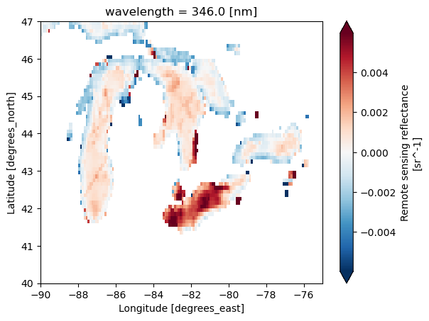
We can plot this object. But let’s not plot the full global data as that is 4+ Gb. We will plot a subset using the slice() function. This way we only load the data needed to plot into memory. We need to

• pick the variable. Let’s use Rrs

• pick a wavelength using sel()

• slice to a smaller lat/lon using slice()

• plot

# Plot
rrs = ds1['Rrs']
rrs346 = rrs.sel(wavelength=346)
rrs346_sub = rrs346.sel(lat=slice(47, 40), lon=slice(-90, -75))
rrs346_sub.plot(robust=True);

# Note this is how we'd usually write this
rrs = ds["Rrs"].sel(
    wavelength=346,
    lat=slice(47, 40),
    lon=slice(-90, -75)
)
rrs.plot(robust=True);

Summary

For Level 3, we use the mapped data product, L3M and the steps to open with xarray are

• earthaccess.search_data() with granule_name to filter to the temporal binning (day, 8-day, month) and resolution (4km or 0.1 degree). We do not need bounding_box since level 3 is global.

• earthaccess.open() to open the search results

• ds=xr.open_dataset(fileset[i]) to open the i-th file in the fileset or ds=xr.open_mfdataset(fileset) to open multiple datasets.

results = earthaccess.search_data(
    short_name = 'PACE_OCI_L3M_RRS',
    temporal = ("2024-03-01", "2025-02-01"),
    granule_name="*.MO.*.0p1deg.*"
)
fileset = earthaccess.open(results)
ds = xr.open_dataset(fileset[1])

Optional. Open all 12 months and make a plot

Open all 12 files with open_mfdataset() and since the netcdf files do not have a time coordinate (just lat, lon, wavelength), we need to tell xarray to combine on a new dimension “time”.

# We can open all the files but note there is no time coordinate so we need
# combine="nested" and concat_dim
ds = xr.open_mfdataset(
    fileset,
    combine="nested",
    concat_dim="time")
ds

<xarray.Dataset> Size: 53GB
Dimensions:     (time: 12, lat: 1800, lon: 3600, wavelength: 172, rgb: 3,
                 eightbitcolor: 256)
Coordinates:
  * wavelength  (wavelength) float64 1kB 346.0 348.0 351.0 ... 714.0 717.0 719.0
  * lat         (lat) float32 7kB 89.95 89.85 89.75 ... -89.75 -89.85 -89.95
  * lon         (lon) float32 14kB -179.9 -179.9 -179.8 ... 179.8 179.9 180.0
Dimensions without coordinates: time, rgb, eightbitcolor
Data variables:
    Rrs         (time, lat, lon, wavelength) float32 53GB dask.array<chunksize=(1, 16, 1024, 8), meta=np.ndarray>
    palette     (time, rgb, eightbitcolor) uint8 9kB dask.array<chunksize=(1, 3, 256), meta=np.ndarray>
Attributes: (12/64)
    product_name:                      PACE_OCI.20240301_20240331.L3m.MO.RRS....
    instrument:                        OCI
    title:                             OCI Level-3 Standard Mapped Image
    project:                           Ocean Biology Processing Group (NASA/G...
    platform:                          PACE
    source:                            satellite observations from OCI-PACE
    ...                                ...
    identifier_product_doi:            10.5067/PACE/OCI/L3M/RRS/3.1
    keywords:                          Earth Science > Oceans > Ocean Optics ...
    keywords_vocabulary:               NASA Global Change Master Directory (G...
    data_bins:                         3315440
    data_minimum:                      -0.009997999
    data_maximum:                      0.09494999

xarray.Dataset

• Dimensions:
  • time: 12
  • lat: 1800
  • lon: 3600
  • wavelength: 172
  • rgb: 3
  • eightbitcolor: 256
• Coordinates: (3)
  • wavelength
    (wavelength)
    float64
    346.0 348.0 351.0 ... 717.0 719.0

    long_name :

    wavelengths

    units :

    nm

    valid_min :

    0

    valid_max :

    20000

    array([346., 348., 351., 353., 356., 358., 361., 363., 366., 368., 371., 373.,
           375., 378., 380., 383., 385., 388., 390., 393., 395., 398., 400., 403.,
           405., 408., 410., 413., 415., 418., 420., 422., 425., 427., 430., 432.,
           435., 437., 440., 442., 445., 447., 450., 452., 455., 457., 460., 462.,
           465., 467., 470., 472., 475., 477., 480., 482., 485., 487., 490., 492.,
           495., 497., 500., 502., 505., 507., 510., 512., 515., 517., 520., 522.,
           525., 527., 530., 532., 535., 537., 540., 542., 545., 547., 550., 553.,
           555., 558., 560., 563., 565., 568., 570., 573., 575., 578., 580., 583.,
           586., 588., 613., 615., 618., 620., 623., 625., 627., 630., 632., 635.,
           637., 640., 641., 642., 643., 645., 646., 647., 648., 650., 651., 652.,
           653., 655., 656., 657., 658., 660., 661., 662., 663., 665., 666., 667.,
           668., 670., 671., 672., 673., 675., 676., 677., 678., 679., 681., 682.,
           683., 684., 686., 687., 688., 689., 691., 692., 693., 694., 696., 697.,
           698., 699., 701., 702., 703., 704., 706., 707., 708., 709., 711., 712.,
           713., 714., 717., 719.])

  • lat
    (lat)
    float32
    89.95 89.85 89.75 ... -89.85 -89.95

    long_name :

    Latitude

    units :

    degrees_north

    standard_name :

    latitude

    valid_min :

    -90.0

    valid_max :

    90.0

    array([ 89.95    ,  89.85    ,  89.75    , ..., -89.75    , -89.850006,
           -89.950005], shape=(1800,), dtype=float32)

  • lon
    (lon)
    float32
    -179.9 -179.9 ... 179.9 180.0

    long_name :

    Longitude

    units :

    degrees_east

    standard_name :

    longitude

    valid_min :

    -180.0

    valid_max :

    180.0

    array([-179.95   , -179.85   , -179.75   , ...,  179.75   ,  179.85   ,
            179.95001], shape=(3600,), dtype=float32)

• Data variables: (2)
  • Rrs
    (time, lat, lon, wavelength)
    float32
    dask.array<chunksize=(1, 16, 1024, 8), meta=np.ndarray>

    long_name :

    Remote sensing reflectance

    units :

    sr^-1

    standard_name :

    surface_ratio_of_upwelling_radiance_emerging_from_sea_water_to_downwelling_radiative_flux_in_air

    valid_min :

    -30000

    valid_max :

    25000

    display_scale :

    linear

    display_min :

    0.0

    display_max :

    0.025

    Array Chunk Bytes 49.82 GiB 512.00 kiB Shape (12, 1800, 3600, 172) (1, 16, 1024, 8) Dask graph 119328 chunks in 37 graph layers Data type float32 numpy.ndarray

  • palette
    (time, rgb, eightbitcolor)
    uint8
    dask.array<chunksize=(1, 3, 256), meta=np.ndarray>

    Array Chunk Bytes 9.00 kiB 768 B Shape (12, 3, 256) (1, 3, 256) Dask graph 12 chunks in 37 graph layers Data type uint8 numpy.ndarray

• Indexes: (3)
  • wavelength
    PandasIndex

    PandasIndex(Index([346.0, 348.0, 351.0, 353.0, 356.0, 358.0, 361.0, 363.0, 366.0, 368.0,
           ...
           706.0, 707.0, 708.0, 709.0, 711.0, 712.0, 713.0, 714.0, 717.0, 719.0],
          dtype='float64', name='wavelength', length=172))

  • lat
    PandasIndex

    PandasIndex(Index([ 89.94999694824219,   89.8499984741211,              89.75,
             89.6500015258789,  89.55000305175781,  89.44999694824219,
             89.3499984741211,              89.25,   89.1500015258789,
            89.05000305175781,
           ...
           -89.05000305175781,  -89.1500015258789,             -89.25,
           -89.35000610351562, -89.45000457763672, -89.55000305175781,
            -89.6500015258789,             -89.75, -89.85000610351562,
           -89.95000457763672],
          dtype='float32', name='lat', length=1800))

  • lon
    PandasIndex

    PandasIndex(Index([ -179.9499969482422, -179.85000610351562,             -179.75,
           -179.64999389648438,  -179.5500030517578,  -179.4499969482422,
           -179.35000610351562,             -179.25, -179.14999389648438,
            -179.0500030517578,
           ...
             179.0500030517578,  179.15000915527344,              179.25,
            179.35000610351562,  179.45001220703125,   179.5500030517578,
            179.65000915527344,              179.75,  179.85000610351562,
            179.95001220703125],
          dtype='float32', name='lon', length=3600))

• Attributes: (64)

  product_name :

  PACE_OCI.20240301_20240331.L3m.MO.RRS.V3_1.Rrs.0p1deg.nc

  instrument :

  OCI

  title :

  OCI Level-3 Standard Mapped Image

  project :

  Ocean Biology Processing Group (NASA/GSFC/OBPG)

  platform :

  PACE

  source :

  satellite observations from OCI-PACE

  temporal_range :

  27-day

  processing_version :

  3.1

  date_created :

  2025-09-22T19:38:45.000Z

  history :

  l3mapgen par=PACE_OCI.20240301_20240331.L3m.MO.RRS.V3_1.Rrs.0p1deg.nc.param

  l2_flag_names :

  ATMFAIL,LAND,HILT,HISATZEN,STRAYLIGHT,CLDICE,COCCOLITH,LOWLW,CHLWARN,CHLFAIL,NAVWARN,MAXAERITER,HISOLZEN,NAVFAIL,FILTER,HIGLINT

  time_coverage_start :

  2024-03-05T00:08:58.225Z

  time_coverage_end :

  2024-04-01T02:24:44.883Z

  start_orbit_number :

  0

  end_orbit_number :

  0

  map_projection :

  Equidistant Cylindrical

  latitude_units :

  degrees_north

  longitude_units :

  degrees_east

  northernmost_latitude :

  90.0

  southernmost_latitude :

  -90.0

  westernmost_longitude :

  -180.0

  easternmost_longitude :

  180.0

  geospatial_lat_max :

  90.0

  geospatial_lat_min :

  -90.0

  geospatial_lon_max :

  180.0

  geospatial_lon_min :

  -180.0

  latitude_step :

  0.1

  longitude_step :

  0.1

  sw_point_latitude :

  -89.95

  sw_point_longitude :

  -179.95

  spatialResolution :

  11.131949 km

  geospatial_lon_resolution :

  11.131949 km

  geospatial_lat_resolution :

  11.131949 km

  geospatial_lat_units :

  degrees_north

  geospatial_lon_units :

  degrees_east

  number_of_lines :

  1800

  number_of_columns :

  3600

  measure :

  Mean

  suggested_image_scaling_minimum :

  0.0

  suggested_image_scaling_maximum :

  0.025

  suggested_image_scaling_type :

  LINEAR

  suggested_image_scaling_applied :

  No

  _lastModified :

  2025-09-22T19:38:45.000Z

  Conventions :

  CF-1.6 ACDD-1.3

  institution :

  NASA Goddard Space Flight Center, Ocean Ecology Laboratory, Ocean Biology Processing Group

  standard_name_vocabulary :

  CF Standard Name Table v36

  naming_authority :

  gov.nasa.gsfc.sci.oceandata

  id :

  3.1/L3/PACE_OCI.20240301_20240331.L3b.MO.RRS.V3_1.nc

  license :

  https://science.nasa.gov/earth-science/earth-science-data/data-information-policy/

  creator_name :

  NASA/GSFC/OBPG

  publisher_name :

  NASA/GSFC/OBPG

  creator_email :

  data@oceancolor.gsfc.nasa.gov

  publisher_email :

  data@oceancolor.gsfc.nasa.gov

  creator_url :

  https://oceandata.sci.gsfc.nasa.gov

  publisher_url :

  https://oceandata.sci.gsfc.nasa.gov

  processing_level :

  L3 Mapped

  cdm_data_type :

  grid

  identifier_product_doi_authority :

  http://dx.doi.org

  identifier_product_doi :

  10.5067/PACE/OCI/L3M/RRS/3.1

  keywords :

  Earth Science > Oceans > Ocean Optics > Reflectance

  keywords_vocabulary :

  NASA Global Change Master Directory (GCMD) Science Keywords

  data_bins :

  3315440

  data_minimum :

  -0.009997999

  data_maximum :

  0.09494999

# Let's add the time coord since we will likely want to subset on time later
import pandas as pd
t = pd.date_range(start="2024-03-01", end="2025-02-01", freq="MS")
ds = ds.assign_coords(time=t)
ds

<xarray.Dataset> Size: 53GB
Dimensions:     (time: 12, lat: 1800, lon: 3600, wavelength: 172, rgb: 3,
                 eightbitcolor: 256)
Coordinates:
  * wavelength  (wavelength) float64 1kB 346.0 348.0 351.0 ... 714.0 717.0 719.0
  * lat         (lat) float32 7kB 89.95 89.85 89.75 ... -89.75 -89.85 -89.95
  * lon         (lon) float32 14kB -179.9 -179.9 -179.8 ... 179.8 179.9 180.0
  * time        (time) datetime64[ns] 96B 2024-03-01 2024-04-01 ... 2025-02-01
Dimensions without coordinates: rgb, eightbitcolor
Data variables:
    Rrs         (time, lat, lon, wavelength) float32 53GB dask.array<chunksize=(1, 16, 1024, 8), meta=np.ndarray>
    palette     (time, rgb, eightbitcolor) uint8 9kB dask.array<chunksize=(1, 3, 256), meta=np.ndarray>
Attributes: (12/64)
    product_name:                      PACE_OCI.20240301_20240331.L3m.MO.RRS....
    instrument:                        OCI
    title:                             OCI Level-3 Standard Mapped Image
    project:                           Ocean Biology Processing Group (NASA/G...
    platform:                          PACE
    source:                            satellite observations from OCI-PACE
    ...                                ...
    identifier_product_doi:            10.5067/PACE/OCI/L3M/RRS/3.1
    keywords:                          Earth Science > Oceans > Ocean Optics ...
    keywords_vocabulary:               NASA Global Change Master Directory (G...
    data_bins:                         3315440
    data_minimum:                      -0.009997999
    data_maximum:                      0.09494999

xarray.Dataset

• Dimensions:
  • time: 12
  • lat: 1800
  • lon: 3600
  • wavelength: 172
  • rgb: 3
  • eightbitcolor: 256
• Coordinates: (4)
  • wavelength
    (wavelength)
    float64
    346.0 348.0 351.0 ... 717.0 719.0

    long_name :

    wavelengths

    units :

    nm

    valid_min :

    0

    valid_max :

    20000

    array([346., 348., 351., 353., 356., 358., 361., 363., 366., 368., 371., 373.,
           375., 378., 380., 383., 385., 388., 390., 393., 395., 398., 400., 403.,
           405., 408., 410., 413., 415., 418., 420., 422., 425., 427., 430., 432.,
           435., 437., 440., 442., 445., 447., 450., 452., 455., 457., 460., 462.,
           465., 467., 470., 472., 475., 477., 480., 482., 485., 487., 490., 492.,
           495., 497., 500., 502., 505., 507., 510., 512., 515., 517., 520., 522.,
           525., 527., 530., 532., 535., 537., 540., 542., 545., 547., 550., 553.,
           555., 558., 560., 563., 565., 568., 570., 573., 575., 578., 580., 583.,
           586., 588., 613., 615., 618., 620., 623., 625., 627., 630., 632., 635.,
           637., 640., 641., 642., 643., 645., 646., 647., 648., 650., 651., 652.,
           653., 655., 656., 657., 658., 660., 661., 662., 663., 665., 666., 667.,
           668., 670., 671., 672., 673., 675., 676., 677., 678., 679., 681., 682.,
           683., 684., 686., 687., 688., 689., 691., 692., 693., 694., 696., 697.,
           698., 699., 701., 702., 703., 704., 706., 707., 708., 709., 711., 712.,
           713., 714., 717., 719.])

  • lat
    (lat)
    float32
    89.95 89.85 89.75 ... -89.85 -89.95

    long_name :

    Latitude

    units :

    degrees_north

    standard_name :

    latitude

    valid_min :

    -90.0

    valid_max :

    90.0

    array([ 89.95    ,  89.85    ,  89.75    , ..., -89.75    , -89.850006,
           -89.950005], shape=(1800,), dtype=float32)

  • lon
    (lon)
    float32
    -179.9 -179.9 ... 179.9 180.0

    long_name :

    Longitude

    units :

    degrees_east

    standard_name :

    longitude

    valid_min :

    -180.0

    valid_max :

    180.0

    array([-179.95   , -179.85   , -179.75   , ...,  179.75   ,  179.85   ,
            179.95001], shape=(3600,), dtype=float32)

  • time
    (time)
    datetime64[ns]
    2024-03-01 ... 2025-02-01

    array(['2024-03-01T00:00:00.000000000', '2024-04-01T00:00:00.000000000',
           '2024-05-01T00:00:00.000000000', '2024-06-01T00:00:00.000000000',
           '2024-07-01T00:00:00.000000000', '2024-08-01T00:00:00.000000000',
           '2024-09-01T00:00:00.000000000', '2024-10-01T00:00:00.000000000',
           '2024-11-01T00:00:00.000000000', '2024-12-01T00:00:00.000000000',
           '2025-01-01T00:00:00.000000000', '2025-02-01T00:00:00.000000000'],
          dtype='datetime64[ns]')

• Data variables: (2)
  • Rrs
    (time, lat, lon, wavelength)
    float32
    dask.array<chunksize=(1, 16, 1024, 8), meta=np.ndarray>

    long_name :

    Remote sensing reflectance

    units :

    sr^-1

    standard_name :

    surface_ratio_of_upwelling_radiance_emerging_from_sea_water_to_downwelling_radiative_flux_in_air

    valid_min :

    -30000

    valid_max :

    25000

    display_scale :

    linear

    display_min :

    0.0

    display_max :

    0.025

    Array Chunk Bytes 49.82 GiB 512.00 kiB Shape (12, 1800, 3600, 172) (1, 16, 1024, 8) Dask graph 119328 chunks in 37 graph layers Data type float32 numpy.ndarray

  • palette
    (time, rgb, eightbitcolor)
    uint8
    dask.array<chunksize=(1, 3, 256), meta=np.ndarray>

    Array Chunk Bytes 9.00 kiB 768 B Shape (12, 3, 256) (1, 3, 256) Dask graph 12 chunks in 37 graph layers Data type uint8 numpy.ndarray

• Indexes: (4)
  • wavelength
    PandasIndex

    PandasIndex(Index([346.0, 348.0, 351.0, 353.0, 356.0, 358.0, 361.0, 363.0, 366.0, 368.0,
           ...
           706.0, 707.0, 708.0, 709.0, 711.0, 712.0, 713.0, 714.0, 717.0, 719.0],
          dtype='float64', name='wavelength', length=172))

  • lat
    PandasIndex

    PandasIndex(Index([ 89.94999694824219,   89.8499984741211,              89.75,
             89.6500015258789,  89.55000305175781,  89.44999694824219,
             89.3499984741211,              89.25,   89.1500015258789,
            89.05000305175781,
           ...
           -89.05000305175781,  -89.1500015258789,             -89.25,
           -89.35000610351562, -89.45000457763672, -89.55000305175781,
            -89.6500015258789,             -89.75, -89.85000610351562,
           -89.95000457763672],
          dtype='float32', name='lat', length=1800))

  • lon
    PandasIndex

    PandasIndex(Index([ -179.9499969482422, -179.85000610351562,             -179.75,
           -179.64999389648438,  -179.5500030517578,  -179.4499969482422,
           -179.35000610351562,             -179.25, -179.14999389648438,
            -179.0500030517578,
           ...
             179.0500030517578,  179.15000915527344,              179.25,
            179.35000610351562,  179.45001220703125,   179.5500030517578,
            179.65000915527344,              179.75,  179.85000610351562,
            179.95001220703125],
          dtype='float32', name='lon', length=3600))

  • time
    PandasIndex

    PandasIndex(DatetimeIndex(['2024-03-01', '2024-04-01', '2024-05-01', '2024-06-01',
                   '2024-07-01', '2024-08-01', '2024-09-01', '2024-10-01',
                   '2024-11-01', '2024-12-01', '2025-01-01', '2025-02-01'],
                  dtype='datetime64[ns]', name='time', freq='MS'))

• Attributes: (64)

  product_name :

  PACE_OCI.20240301_20240331.L3m.MO.RRS.V3_1.Rrs.0p1deg.nc

  instrument :

  OCI

  title :

  OCI Level-3 Standard Mapped Image

  project :

  Ocean Biology Processing Group (NASA/GSFC/OBPG)

  platform :

  PACE

  source :

  satellite observations from OCI-PACE

  temporal_range :

  27-day

  processing_version :

  3.1

  date_created :

  2025-09-22T19:38:45.000Z

  history :

  l3mapgen par=PACE_OCI.20240301_20240331.L3m.MO.RRS.V3_1.Rrs.0p1deg.nc.param

  l2_flag_names :

  ATMFAIL,LAND,HILT,HISATZEN,STRAYLIGHT,CLDICE,COCCOLITH,LOWLW,CHLWARN,CHLFAIL,NAVWARN,MAXAERITER,HISOLZEN,NAVFAIL,FILTER,HIGLINT

  time_coverage_start :

  2024-03-05T00:08:58.225Z

  time_coverage_end :

  2024-04-01T02:24:44.883Z

  start_orbit_number :

  0

  end_orbit_number :

  0

  map_projection :

  Equidistant Cylindrical

  latitude_units :

  degrees_north

  longitude_units :

  degrees_east

  northernmost_latitude :

  90.0

  southernmost_latitude :

  -90.0

  westernmost_longitude :

  -180.0

  easternmost_longitude :

  180.0

  geospatial_lat_max :

  90.0

  geospatial_lat_min :

  -90.0

  geospatial_lon_max :

  180.0

  geospatial_lon_min :

  -180.0

  latitude_step :

  0.1

  longitude_step :

  0.1

  sw_point_latitude :

  -89.95

  sw_point_longitude :

  -179.95

  spatialResolution :

  11.131949 km

  geospatial_lon_resolution :

  11.131949 km

  geospatial_lat_resolution :

  11.131949 km

  geospatial_lat_units :

  degrees_north

  geospatial_lon_units :

  degrees_east

  number_of_lines :

  1800

  number_of_columns :

  3600

  measure :

  Mean

  suggested_image_scaling_minimum :

  0.0

  suggested_image_scaling_maximum :

  0.025

  suggested_image_scaling_type :

  LINEAR

  suggested_image_scaling_applied :

  No

  _lastModified :

  2025-09-22T19:38:45.000Z

  Conventions :

  CF-1.6 ACDD-1.3

  institution :

  NASA Goddard Space Flight Center, Ocean Ecology Laboratory, Ocean Biology Processing Group

  standard_name_vocabulary :

  CF Standard Name Table v36

  naming_authority :

  gov.nasa.gsfc.sci.oceandata

  id :

  3.1/L3/PACE_OCI.20240301_20240331.L3b.MO.RRS.V3_1.nc

  license :

  https://science.nasa.gov/earth-science/earth-science-data/data-information-policy/

  creator_name :

  NASA/GSFC/OBPG

  publisher_name :

  NASA/GSFC/OBPG

  creator_email :

  data@oceancolor.gsfc.nasa.gov

  publisher_email :

  data@oceancolor.gsfc.nasa.gov

  creator_url :

  https://oceandata.sci.gsfc.nasa.gov

  publisher_url :

  https://oceandata.sci.gsfc.nasa.gov

  processing_level :

  L3 Mapped

  cdm_data_type :

  grid

  identifier_product_doi_authority :

  http://dx.doi.org

  identifier_product_doi :

  10.5067/PACE/OCI/L3M/RRS/3.1

  keywords :

  Earth Science > Oceans > Ocean Optics > Reflectance

  keywords_vocabulary :

  NASA Global Change Master Directory (GCMD) Science Keywords

  data_bins :

  3315440

  data_minimum :

  -0.009997999

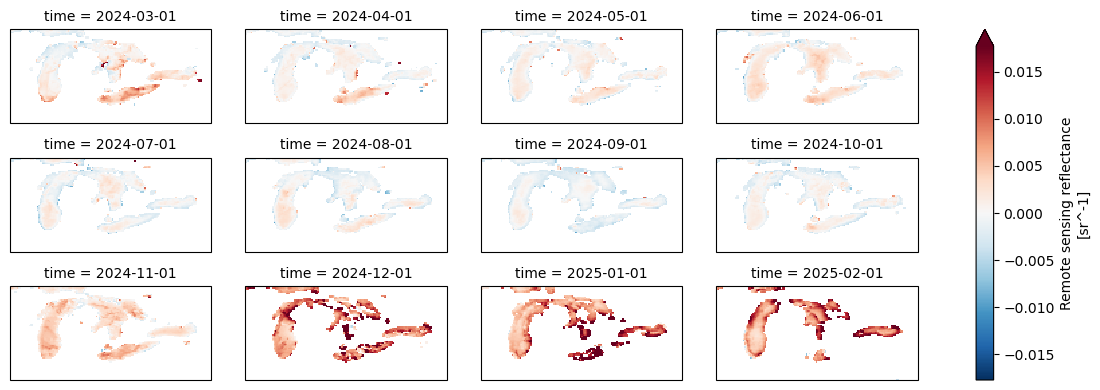
  data_maximum :

  0.09494999

Let’s plot all the months and fix the warping of space by adding a lat/lon projection, aka tell the plotting that this is lat/lon on a globe.

rrs = ds["Rrs"].sel(
    wavelength=346,
    lat=slice(47, 40),
    lon=slice(-90, -75)
)

import cartopy.crs as ccrs
rrs.plot(
    col="time",            # one panel per month
    col_wrap=4,            # 4 columns per row
    robust=True,           # ignore outliers for color scale
    figsize=(12, 4),
    subplot_kws={"projection": ccrs.PlateCarree()},
    transform=ccrs.PlateCarree()
)

<xarray.plot.facetgrid.FacetGrid at 0x7f413816ec90>

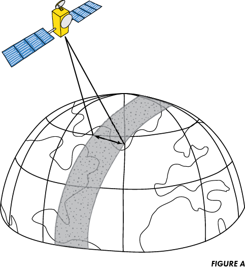
Level 2 data

Level 2 data is not on a global lat/lon grid. Instead each swath (satelite path) has “lines” along the path and “pixels” across the lines (perpendicular to path). In addition, the data files are GROUPED netcdfs (different format). We need to open these with open_datatree and then merge all the groups.

Let’s get the swath(s) over the U.S. Great Lakes on March 5th, 2025.

import xarray as xr
import earthaccess
auth = earthaccess.login(persist=True)
results = earthaccess.search_data(
    short_name = 'PACE_OCI_L2_AOP',
    temporal = ("2025-03-05", "2025-03-05"),
    bounding_box = (-90.0, 40.0, -75.0, 47.0)
)
len(results) # one of this is a monthly average

3

# Step 1 set up the fileset
fileset = earthaccess.open(results)

# Step 2 open L2 swath files with xarray open_datatree
datatree = xr.open_datatree(fileset[1], decode_timedelta=False) 
datatree.groups

('/',
 '/sensor_band_parameters',
 '/scan_line_attributes',
 '/geophysical_data',
 '/navigation_data',
 '/processing_control',
 '/processing_control/input_parameters',
 '/processing_control/flag_percentages')

The geophysical data is the data like Rrs and the navigation data has the lat/lon information for each line/pixel.

# Step 3 merge the groups all together.
# This works due to the values in each group being the same shape.
ds_l2 = xr.merge(datatree.to_dict().values())
ds_l2 = ds_l2.set_coords(("longitude", "latitude"))
ds_l2

<xarray.Dataset> Size: 3GB
Dimensions:        (number_of_bands: 286, number_of_reflective_bands: 286,
                    wavelength_3d: 172, number_of_lines: 1710,
                    pixels_per_line: 1272)
Coordinates:
  * wavelength_3d  (wavelength_3d) float64 1kB 346.0 348.0 351.0 ... 717.0 719.0
    longitude      (number_of_lines, pixels_per_line) float32 9MB ...
    latitude       (number_of_lines, pixels_per_line) float32 9MB ...
Dimensions without coordinates: number_of_bands, number_of_reflective_bands,
                                number_of_lines, pixels_per_line
Data variables: (12/30)
    wavelength     (number_of_bands) float64 2kB ...
    vcal_gain      (number_of_reflective_bands) float32 1kB ...
    vcal_offset    (number_of_reflective_bands) float32 1kB ...
    F0             (number_of_reflective_bands) float32 1kB ...
    aw             (number_of_reflective_bands) float32 1kB ...
    bbw            (number_of_reflective_bands) float32 1kB ...
    ...             ...
    aot_865        (number_of_lines, pixels_per_line) float32 9MB ...
    angstrom       (number_of_lines, pixels_per_line) float32 9MB ...
    avw            (number_of_lines, pixels_per_line) float32 9MB ...
    nflh           (number_of_lines, pixels_per_line) float32 9MB ...
    l2_flags       (number_of_lines, pixels_per_line) int32 9MB ...
    tilt           (number_of_lines) float32 7kB ...
Attributes: (12/47)
    title:                             OCI Level-2 Data AOP
    product_name:                      PACE_OCI.20250305T174755.L2.OC_AOP.V3_...
    processing_version:                3.1
    history:                           l2gen par=/data3/sdpsoper/vdc/vpu22/wo...
    instrument:                        OCI
    platform:                          PACE
    ...                                ...
    geospatial_lon_min:                -102.731316
    startDirection:                    Ascending
    endDirection:                      Ascending
    day_night_flag:                    Day
    earth_sun_distance_correction:     1.0163003206253052
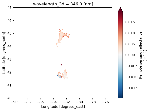
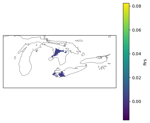
    geospatial_bounds:                 POLYGON ((-63.58643 55.76101, -102.731...

xarray.Dataset

• Dimensions:
  • number_of_bands: 286
  • number_of_reflective_bands: 286
  • wavelength_3d: 172
  • number_of_lines: 1710
  • pixels_per_line: 1272
• Coordinates: (3)
  • wavelength_3d
    (wavelength_3d)
    float64
    346.0 348.0 351.0 ... 717.0 719.0

    long_name :

    wavelengths

    units :

    nm

    valid_min :

    0

    valid_max :

    20000

    array([346., 348., 351., 353., 356., 358., 361., 363., 366., 368., 371., 373.,
           375., 378., 380., 383., 385., 388., 390., 393., 395., 398., 400., 403.,
           405., 408., 410., 413., 415., 418., 420., 422., 425., 427., 430., 432.,
           435., 437., 440., 442., 445., 447., 450., 452., 455., 457., 460., 462.,
           465., 467., 470., 472., 475., 477., 480., 482., 485., 487., 490., 492.,
           495., 497., 500., 502., 505., 507., 510., 512., 515., 517., 520., 522.,
           525., 527., 530., 532., 535., 537., 540., 542., 545., 547., 550., 553.,
           555., 558., 560., 563., 565., 568., 570., 573., 575., 578., 580., 583.,
           586., 588., 613., 615., 618., 620., 623., 625., 627., 630., 632., 635.,
           637., 640., 641., 642., 643., 645., 646., 647., 648., 650., 651., 652.,
           653., 655., 656., 657., 658., 660., 661., 662., 663., 665., 666., 667.,
           668., 670., 671., 672., 673., 675., 676., 677., 678., 679., 681., 682.,
           683., 684., 686., 687., 688., 689., 691., 692., 693., 694., 696., 697.,
           698., 699., 701., 702., 703., 704., 706., 707., 708., 709., 711., 712.,
           713., 714., 717., 719.])

  • longitude
    (number_of_lines, pixels_per_line)
    float32
    ...

    long_name :

    Longitude

    units :

    degrees_east

    standard_name :

    longitude

    valid_min :

    -180.0

    valid_max :

    180.0

    [2175120 values with dtype=float32]

  • latitude
    (number_of_lines, pixels_per_line)
    float32
    ...

    long_name :

    Latitude

    units :

    degrees_north

    standard_name :

    latitude

    valid_min :

    -90.0

    valid_max :

    90.0

    [2175120 values with dtype=float32]

• Data variables: (30)
  • wavelength
    (number_of_bands)
    float64
    ...

    long_name :

    wavelengths

    units :

    nm

    valid_min :

    0

    valid_max :

    20000

    [286 values with dtype=float64]

  • vcal_gain
    (number_of_reflective_bands)
    float32
    ...

    long_name :

    Vicarious Calibration Gain

    valid_min :

    0.0

    valid_max :

    2.0

    [286 values with dtype=float32]

  • vcal_offset
    (number_of_reflective_bands)
    float32
    ...

    long_name :

    Vicarious Calibration Offset

    units :

    mW cm^-2 um^-1 sr^-1

    valid_min :

    0.0

    valid_max :

    10.0

    [286 values with dtype=float32]

  • F0
    (number_of_reflective_bands)
    float32
    ...

    long_name :

    Mean Solar Flux

    units :

    W m^-2 um^-1

    valid_min :

    0.0

    valid_max :

    2500.0

    [286 values with dtype=float32]

  • aw
    (number_of_reflective_bands)
    float32
    ...

    long_name :

    Band-pass averaged absorption coefficient for seawater

    units :

    m^-1

    standard_name :

    volume_absorption_coefficient_of_radiative_flux_in_sea_water

    valid_min :

    1e-04

    valid_max :

    5.0

    reference :

    Pope, R.M. and Fry, E.S., 1997, "Absorption spectrum (380-700 nm) of pure water. II. Integrating cavity measurements," Appl. Opt.,36, 8710-8723.; Kou, L., Labrie, D., Chylek, P., 1993, "Refractive indices of water and ice in the 0.65-2.5 m spectral range," Appl. Opt.,32, 3531-3540 (1993).

    [286 values with dtype=float32]

  • bbw
    (number_of_reflective_bands)
    float32
    ...

    long_name :

    Band-pass averaged backscattering coefficient for seawater

    units :

    m^-1

    standard_name :

    volume_backwards_scattering_coefficient_of_radiative_flux_in_sea_water

    valid_min :

    5e-06

    valid_max :

    1.0

    reference :

    Zhang, X., Hu, L., and He, M.-X. (2009). Scattering by pure seawater: effect of salinity, Opt. Express 17(7)

    comment :

    These are nominal values for a salinity of 38.4 at 20 degrees C. The bbw values used in the processing are corrected for temperature and salinity on a per pixel basis.

    [286 values with dtype=float32]

  • k_oz
    (number_of_reflective_bands)
    float32
    ...

    long_name :

    Ozone Absorption cross-sections

    units :

    cm^-1

    valid_min :

    0.0

    valid_max :

    0.1

    reference :

    Anderson, S.M., Morton, J., and Mauersberger, K. "Near-infrared absorption spectra of 16O3 and 18O3: Adiabatic energy of the 1A2 state?." The Journal of Chemical Physics 93.6 (1990): 3826-3832.; Anderson, Stuart M., Maeder, J., and Mauersberger, K. "Effect of isotopic substitution on the visible absorption spectrum of ozone." The Journal of chemical physics 94.10 (1991): 6351-6357; http://dx.doi.org/10.1029/92GL00780; http://dx.doi.org/10.1029/93GL01765; http://dx.doi.org/10.1029/93GL02311

    comment :

    Computed at 229.15K with code provided by E.P.Shettle, NRL, Washington, DC; Based on the measurements of: S.Anderson et al. and J. Burkholder and Talukdar (1994)

    [286 values with dtype=float32]

  • k_no2
    (number_of_reflective_bands)
    float32
    ...

    long_name :

    NO2 Absorption cross-sections

    units :

    cm^2 molecule^-1

    valid_min :

    0.0

    valid_max :

    0.1

    reference :

    K. Bogumil, et al., "Measurements of molecular absorption spectra with the SCIAMACHY pre-flight model: Instrument characterization and reference data for atmospheric remote sensing in the 230-2380 nm region," J. Photochem. Photobiol. A.: Photochem. 157, 167-184 (2003).; W. Schneider,et al., "Absorption cross-sections of NO2 in the UV and visible region (200 - 700 nm) at 298 K", J. Photochem. Photobiol. 40, 195-217 (1987)

    [286 values with dtype=float32]

  • Tau_r
    (number_of_reflective_bands)
    float32
    ...

    long_name :

    Rayleigh Optical Thickness

    valid_min :

    0.0

    valid_max :

    0.5

    reference :

    Bodhaine, B.A., Wood, N.B, Dutton, E.G., Slusser, J.R. (1999). On Rayleigh Optical Depth Calculations, J. Atmos. Ocean Tech., 16, 1854-1861.

    [286 values with dtype=float32]

  • year
    (number_of_lines)
    float64
    ...

    long_name :

    Scan year

    units :

    years

    valid_min :

    1900

    valid_max :

    2100

    [1710 values with dtype=float64]

  • day
    (number_of_lines)
    float64
    ...

    long_name :

    Scan day of year

    units :

    days

    valid_min :

    0

    valid_max :

    366

    [1710 values with dtype=float64]

  • msec
    (number_of_lines)
    float64
    ...

    long_name :

    Scan time, milliseconds of day

    units :

    milliseconds

    valid_min :

    0

    valid_max :

    86400000

    [1710 values with dtype=float64]

  • time
    (number_of_lines)
    datetime64[ns]
    ...

    long_name :

    scan line time in seconds since 1970-1-1

    [1710 values with dtype=datetime64[ns]]

  • detnum
    (number_of_lines)
    float32
    ...

    long_name :

    Detector Number (zero-based)

    valid_min :

    0

    valid_max :

    25

    [1710 values with dtype=float32]

  • mside
    (number_of_lines)
    float32
    ...

    long_name :

    Mirror Side (zero-based)

    valid_min :

    0

    valid_max :

    1

    [1710 values with dtype=float32]

  • slon
    (number_of_lines)
    float32
    ...

    long_name :

    Starting Longitude

    units :

    degrees_east

    standard_name :

    longitude

    valid_min :

    -180.0

    valid_max :

    180.0

    [1710 values with dtype=float32]

  • clon
    (number_of_lines)
    float32
    ...

    long_name :

    Center Longitude

    units :

    degrees_east

    standard_name :

    longitude

    valid_min :

    -180.0

    valid_max :

    180.0

    [1710 values with dtype=float32]

  • elon
    (number_of_lines)
    float32
    ...

    long_name :

    Ending Longitude

    units :

    degrees_east

    standard_name :

    longitude

    valid_min :

    -180.0

    valid_max :

    180.0

    [1710 values with dtype=float32]

  • slat
    (number_of_lines)
    float32
    ...

    long_name :

    Starting Latitude

    units :

    degrees_north

    standard_name :

    latitude

    valid_min :

    -90.0

    valid_max :

    90.0

    [1710 values with dtype=float32]

  • clat
    (number_of_lines)
    float32
    ...

    long_name :

    Center Latitude

    units :

    degrees_north

    standard_name :

    latitude

    valid_min :

    -90.0

    valid_max :

    90.0

    [1710 values with dtype=float32]

  • elat
    (number_of_lines)
    float32
    ...

    long_name :

    Ending Latitude

    units :

    degrees_north

    standard_name :

    latitude

    valid_min :

    -90.0

    valid_max :

    90.0

    [1710 values with dtype=float32]

  • csol_z
    (number_of_lines)
    float32
    ...

    long_name :

    Center Solar Zenith Angle

    units :

    degree

    valid_min :

    -90.0

    valid_max :

    90.0

    [1710 values with dtype=float32]

  • Rrs
    (number_of_lines, pixels_per_line, wavelength_3d)
    float32
    ...

    long_name :

    Remote sensing reflectance

    units :

    sr^-1

    standard_name :

    surface_ratio_of_upwelling_radiance_emerging_from_sea_water_to_downwelling_radiative_flux_in_air

    valid_min :

    -30000

    valid_max :

    25000

    [374120640 values with dtype=float32]

  • Rrs_unc
    (number_of_lines, pixels_per_line, wavelength_3d)
    float32
    ...

    long_name :

    Uncertainty in remote sensing reflectance

    units :

    sr^-1

    valid_min :

    -30000

    valid_max :

    30000

    [374120640 values with dtype=float32]

  • aot_865
    (number_of_lines, pixels_per_line)
    float32
    ...

    long_name :

    Aerosol optical thickness at 865 nm

    standard_name :

    atmosphere_optical_thickness_due_to_ambient_aerosol

    valid_min :

    0

    valid_max :

    30000

    [2175120 values with dtype=float32]

  • angstrom
    (number_of_lines, pixels_per_line)
    float32
    ...

    long_name :

    Aerosol Angstrom exponent, 443 to 865 nm

    standard_name :

    aerosol_angstrom_exponent

    valid_min :

    -30000

    valid_max :

    5000

    [2175120 values with dtype=float32]

  • avw
    (number_of_lines, pixels_per_line)
    float32
    ...

    long_name :

    Apparent Visible Wavelength

    units :

    nm

    valid_min :

    400.0

    valid_max :

    700.0

    reference :

    Vandermeulen, R. A., Mannino, A., Craig, S.E., Werdell, P.J., 2020: 150 shades of green: Using the full spectrum of remote sensing reflectance to elucidate color shifts in the ocean, Remote Sensing of Environment, 247, 111900, https://doi.org/10.1016/j.rse.2020.111900, https://doi.org/10.5067/KAROCHG01RYJ

    [2175120 values with dtype=float32]

  • nflh
    (number_of_lines, pixels_per_line)
    float32
    ...

    long_name :

    Normalized Fluorescence Line Height

    units :

    W m^-2 um^-1 sr^-1

    valid_min :

    -26471

    valid_max :

    32353

    reference :

    Behrenfeld, M.J., Westberry, T.K., Boss, E.S., O'Malley, R.T., Siegel, D.A., Wiggert, J.D., Franz, B.A., McClain, C.R., Feldman, G.C., Doney, S.C., Moore, J.K., Dall'Olmo, G., Milligan, A.J., Lima, I., and Mahowald, N.: Satellite-detected fluorescence reveals global physiology of ocean phytoplankton, Biogeosciences, 6, 779-794, doi:10.5194/bg-6-779-2009, 2009.

    [2175120 values with dtype=float32]

  • l2_flags
    (number_of_lines, pixels_per_line)
    int32
    ...

    long_name :

    Level-2 Processing Flags

    valid_min :

    -2147483648

    valid_max :

    2147483647

    flag_masks :

    [ 1 2 4 8 16 32 64 128 256 512 1024 2048 4096 8192 16384 32768 65536 131072 262144 524288 1048576 2097152 4194304 8388608 16777216 33554432 67108864 134217728 268435456 536870912 1073741824 -2147483648]

    flag_meanings :

    ATMFAIL LAND PRODWARN HIGLINT HILT HISATZEN COASTZ SPARE STRAYLIGHT CLDICE COCCOLITH TURBIDW HISOLZEN SPARE LOWLW CHLFAIL NAVWARN ABSAER SPARE MAXAERITER MODGLINT CHLWARN ATMWARN OPSHAL SEAICE NAVFAIL FILTER SPARE BOWTIEDEL HIPOL PRODFAIL SPARE

    [2175120 values with dtype=int32]

  • tilt
    (number_of_lines)
    float32
    ...

    long_name :

    Sensor tilt angle

    units :

    degree

    valid_min :

    -25.0

    valid_max :

    25.0

    [1710 values with dtype=float32]

• Indexes: (1)
  • wavelength_3d
    PandasIndex

    PandasIndex(Index([346.0, 348.0, 351.0, 353.0, 356.0, 358.0, 361.0, 363.0, 366.0, 368.0,
           ...
           706.0, 707.0, 708.0, 709.0, 711.0, 712.0, 713.0, 714.0, 717.0, 719.0],
          dtype='float64', name='wavelength_3d', length=172))

• Attributes: (47)

  title :

  OCI Level-2 Data AOP

  product_name :

  PACE_OCI.20250305T174755.L2.OC_AOP.V3_1.nc

  processing_version :

  3.1

  history :

  l2gen par=/data3/sdpsoper/vdc/vpu22/workbuf/PACE_OCI.20250305T174755.L1B.V3.nc.param metafile=PACE_OCI.20250305T174755.L2.OC_AOP.V3_1.nc.meta

  instrument :

  OCI

  platform :

  PACE

  Conventions :

  CF-1.8, ACDD-1.3

  license :

  https://science.nasa.gov/earth-science/earth-science-data/data-information-policy/

  naming_authority :

  gov.nasa.gsfc.sci.oceandata

  id :

  3.1/L2/PACE_OCI.20250305T174755.L2.OC_AOP.V3_1.nc

  date_created :

  2025-09-20T05:37:38.000Z

  standard_name_vocabulary :

  CF Standard Name Table v36

  institution :

  NASA Goddard Space Flight Center, Ocean Ecology Laboratory, Ocean Biology Processing Group

  creator_name :

  NASA/GSFC/OBPG

  creator_email :

  data@oceancolor.gsfc.nasa.gov

  creator_url :

  https://oceandata.sci.gsfc.nasa.gov

  project :

  Ocean Biology Processing Group (NASA/GSFC/OBPG)

  publisher_name :

  NASA/GSFC/OBPG

  publisher_url :

  https://oceandata.sci.gsfc.nasa.gov

  publisher_email :

  data@oceancolor.gsfc.nasa.gov

  geospatial_bounds_crs :

  EPSG:4326

  identifier_product_doi_authority :

  http://dx.doi.org

  identifier_product_doi :

  10.5067/PACE/OCI/L2/OC_AOP/3.1

  processing_level :

  L2

  cdm_data_type :

  swath

  spatialResolution :

  1000 m

  time_coverage_start :

  2025-03-05T17:47:55.118Z

  time_coverage_end :

  2025-03-05T17:52:55.000Z

  start_center_longitude :

  -77.95977

  start_center_latitude :

  35.590504

  end_center_longitude :

  -84.4568

  end_center_latitude :

  53.552963

  northernmost_latitude :

  55.761013

  southernmost_latitude :

  32.448944

  easternmost_longitude :

  -63.058395

  westernmost_longitude :

  -102.731316

  geospatial_lat_units :

  degrees_north

  geospatial_lon_units :

  degrees_east

  geospatial_lat_max :

  55.761013

  geospatial_lat_min :

  32.448944

  geospatial_lon_max :

  -63.058395

  geospatial_lon_min :

  -102.731316

  startDirection :

  Ascending

  endDirection :

  Ascending

  day_night_flag :

  Day

  earth_sun_distance_correction :

  1.0163003206253052

  geospatial_bounds :

  POLYGON ((-63.58643 55.76101, -102.73132 49.13079, -92.11572 32.44894, -63.05840 38.01264, -63.58643 55.76101))

Let’s plot. Hmm it’s mainly blank. This is daily swath data. There were lots of clouds that day or the swath only included part of region.

• Specify the variable Rrs in [ ]

• Spefify the wavelength, a coordinate, using .sel()

• Plot and tell it to use longitude for x and latitude for y.

# Plot
rrs = ds_l2['Rrs'].sel(
    wavelength_3d=346)
rrs.plot(robust=True, 
         x="longitude", y="latitude",
         xlim=(-90, -75), ylim=(40, 47));

Optional. Plot with the outline of the Great Lakes

import matplotlib.pyplot as plt
import cartopy.crs as ccrs
import cartopy.feature as cfeature

fig = plt.figure(figsize=(6,5))
ax = plt.axes(projection=ccrs.PlateCarree())
ax.set_extent([-90, -75, 40, 47], crs=ccrs.PlateCarree())
ax.add_feature(cfeature.LAKES.with_scale("50m"),
               facecolor="none", edgecolor="grey", linewidth=0.8)

# swath pieces
da  = ds_l2["Rrs"].sel(wavelength_3d=346)     # (lines, pixels)
lat = ds_l2["latitude"]
lon = ds_l2["longitude"]

# add to your existing ax (before plt.show)
im = ax.pcolormesh(
    lon, lat, da,
    transform=ccrs.PlateCarree(),
    shading="nearest",      # lighter than 'auto'
    rasterized=True
)
plt.colorbar(im, ax=ax, label="Rrs")

plt.show()

Summary

With level 2 data, we need to use xarray.open_datatree() and then do a merge step to get all the variables in the groups. Note we can only work with one level 2 dataset at a time.

• res=earthaccess.search_data() with bounding_box to filter to the region of interest.

• fileset=earthaccess.open(res)

• datatree=xarray.open_datatree(fileset[i]) to open the i-th file in the fileset.

• ds=xarray.merge(datatree.to_dict().values()) to merge all the groups

• ds = ds.set_coords(("longitude", "latitude")) to make longitude and latitude coords (will help with plotting.

# Get L2 data
results = earthaccess.search_data(
    short_name = 'PACE_OCI_L2_AOP',
    temporal = ("2025-03-05", "2025-03-05"),
    bounding_box = (-90.0, 40.0, -75.0, 47.0)
)
fileset = earthaccess.open(results)

# Open with the grouped netCDFs with open_datatree
datatree = xr.open_datatree(fileset[1], decode_timedelta=False)
ds_l2 = xr.merge(datatree.to_dict().values())
ds_l2 = ds_l2.set_coords(("longitude", "latitude"))
ds_l2

Working with larger than memory data

Here are a few basics to know when working with larger-than memory data.

Chunks

The PACE data are cloud-optimized (read optimized) so that we don’t have to read the whole file into memory to work with it and we don’t have to download the whole thing if we don’t need to.

import earthaccess
import xarray as xr
results = earthaccess.search_data(
    short_name = 'PACE_OCI_L3M_RRS',
    temporal = ("2024-03-01", "2025-04-01"),
    granule_name="*.MO.*.0p1deg.*"
)
fileset = earthaccess.open(results)

# this creates a chunked reference to our data that we can load chunk by chunk
ds_chunk = xr.open_dataset(fileset[0], chunks={})
# this creates a reference that we have to load in its entirety
ds = xr.open_dataset(fileset[0])

ds_size_gb = ds.nbytes / 1e9
print(f"Dataset size: {ds_size_gb:.2f} GB")

Dataset size: 4.46 GB

# Check that ds_chunk is chunked
ds_chunk.chunks

Frozen({'lat': (16, 16, 16, 16, 16, 16, 16, 16, 16, 16, 16, 16, 16, 16, 16, 16, 16, 16, 16, 16, 16, 16, 16, 16, 16, 16, 16, 16, 16, 16, 16, 16, 16, 16, 16, 16, 16, 16, 16, 16, 16, 16, 16, 16, 16, 16, 16, 16, 16, 16, 16, 16, 16, 16, 16, 16, 16, 16, 16, 16, 16, 16, 16, 16, 16, 16, 16, 16, 16, 16, 16, 16, 16, 16, 16, 16, 16, 16, 16, 16, 16, 16, 16, 16, 16, 16, 16, 16, 16, 16, 16, 16, 16, 16, 16, 16, 16, 16, 16, 16, 16, 16, 16, 16, 16, 16, 16, 16, 16, 16, 16, 16, 8), 'lon': (1024, 1024, 1024, 528), 'wavelength': (8, 8, 8, 8, 8, 8, 8, 8, 8, 8, 8, 8, 8, 8, 8, 8, 8, 8, 8, 8, 8, 4), 'rgb': (3,), 'eightbitcolor': (256,)})

# but ds is not chunked
ds.chunks

Frozen({})

Chunking allows operations on bigger than memory datasets

Chunking let’s us work with big datasets without blowing up our memory. This task takes awhile but it doesn’t blow up our little 2Gb RAM virtual machines. xarray and dask are smart and work through the task chunk by chunk. Downside is that the chunked dataset is chunked into little chunks which mean a lot of queries to the cloud data to read each little chunk. That means it will be very slow.

%%time
# ds is not chunked
# This loads a 200 Mb array at once. Watch below how the memory increases (if on a JupyterHub)
var = ds["Rrs"].isel(wavelength=slice(1,9))
global_mean = var.mean().values

CPU times: user 15.3 s, sys: 7.04 s, total: 22.4 s
Wall time: 1min 13s

%%time
# ds_chunk is chunked into little chunks
# This can be done chunk by chunk and will increase the memory usage much since chunks are tiny, but slow.
var = ds_chunk["Rrs"].isel(wavelength=slice(1,9))
global_mean = var.mean().values

CPU times: user 7.2 s, sys: 1.19 s, total: 8.39 s
Wall time: 2min 21s

Working with Larger-Than-Memory Data When You Cannot Change Chunk Sizes

In the case of the PACE data, the chunk sizes are small and computations are much slower than if we could load all the data into memory but we don’t blow up the memory so we can work with big files on machines with minimal RAM or with lots of little dask workers in a big RAM machine.

When datasets are stored in the cloud with very small physical chunks, the key is to design computations that minimize repeated remote reads and avoid loading the full array into RAM. Even though the tiny chunking slows down global operations, Dask + Xarray can still handle larger-than-memory workflows efficiently if you structure your analysis around streaming, subsetting, and locality or we can use a non-chunked dataset if we only load in smaller than memory subsets.

Practical Tips

• Always subset to your region and time of interest before working with your dataset. So sel() and isel() before mean() or var(). Focus only on the wavelengths and variables of interest (so use like ds["Rrs"] to get just that variable).

• Avoid operations that require full materialization such as .load() or .values on large arrays. Instead, keep arrays lazy and call .compute() only on reduced results (e.g., monthly means, statistics, anomalies), which keeps memory usage bounded.

• Use xarray.open_data(..., chunks={}) to create a version of your data that has the chunk references if you need to make sure memory use is limited. This is going to be slower, but won’t blow up memory. Use ds.chunks() on your xarray dataset to find out if the dataset is chunked or not.

• .plot() will load all the data so make sure to plot smaller regions. hvplot() uses dask if you want to plot something that is larger than memory.

• Coding LLMs (Claude, ChatGPT) are very helpful in debugging memory issues and chunking issues.

• If you need to run computations with dask, use a machine with big memory and lots of workers because your chunks are small and each worker doesn’t need too much memory. But you will likely be limited by the number of http connections you can make (since the bottleneck in cloud data is often the I/O calls).

Summary

This concludes the earthaccess tutorial for PACE data.

• Opening Level 3 netcdfs with xarray

• Opening Level 2 netcdfs with xarray and datatree

• Working with larger than memory data.