Inferring Global Chlorophyll-a Depth Profiles from PACE Hyperspectral Rrs
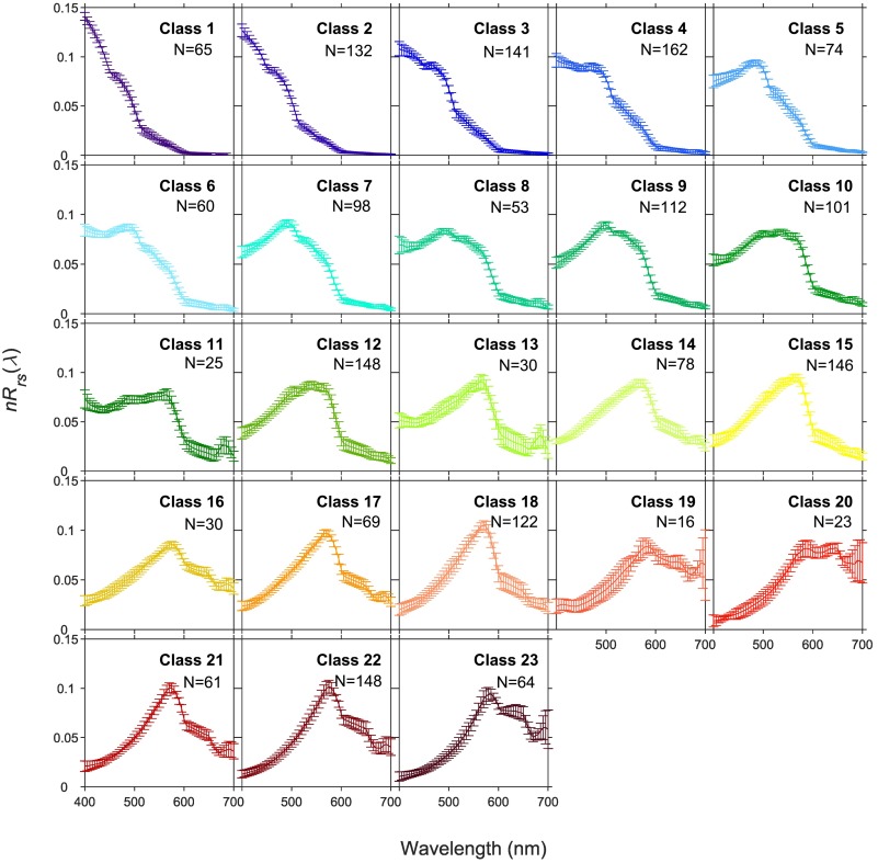
What Does Hyperspectral Rrs Look Like Compared to Multi-Spectral?
Results spoiler. It works!
Caveat: Mostly trained on data from open ocean (BGC-Argo). Most data was for surface CHLA < 1. Need more coastal data. Though it does do a decent job for the surface CHLA > 10 data that we do have.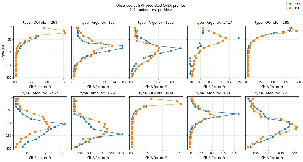
BGC-Argo
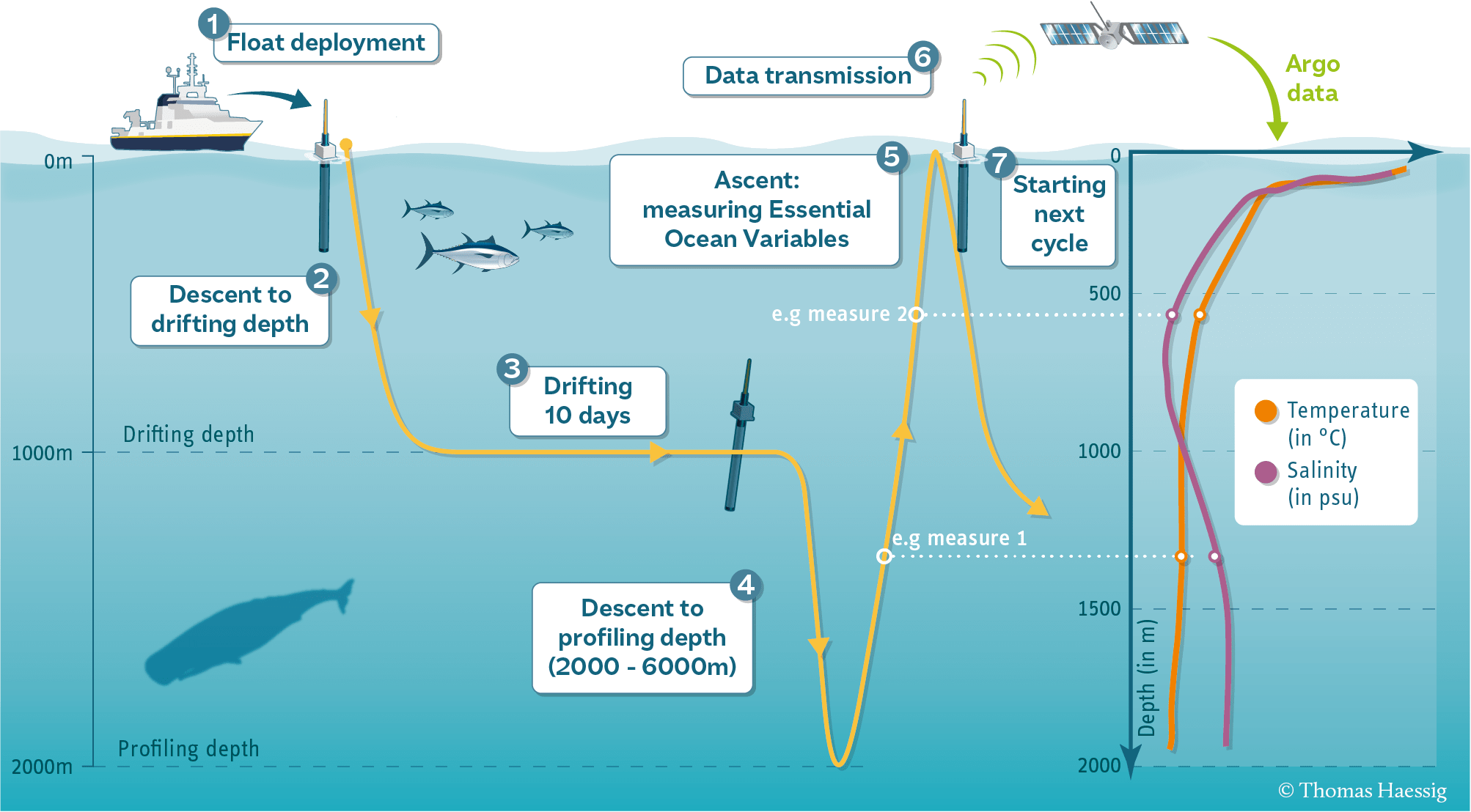
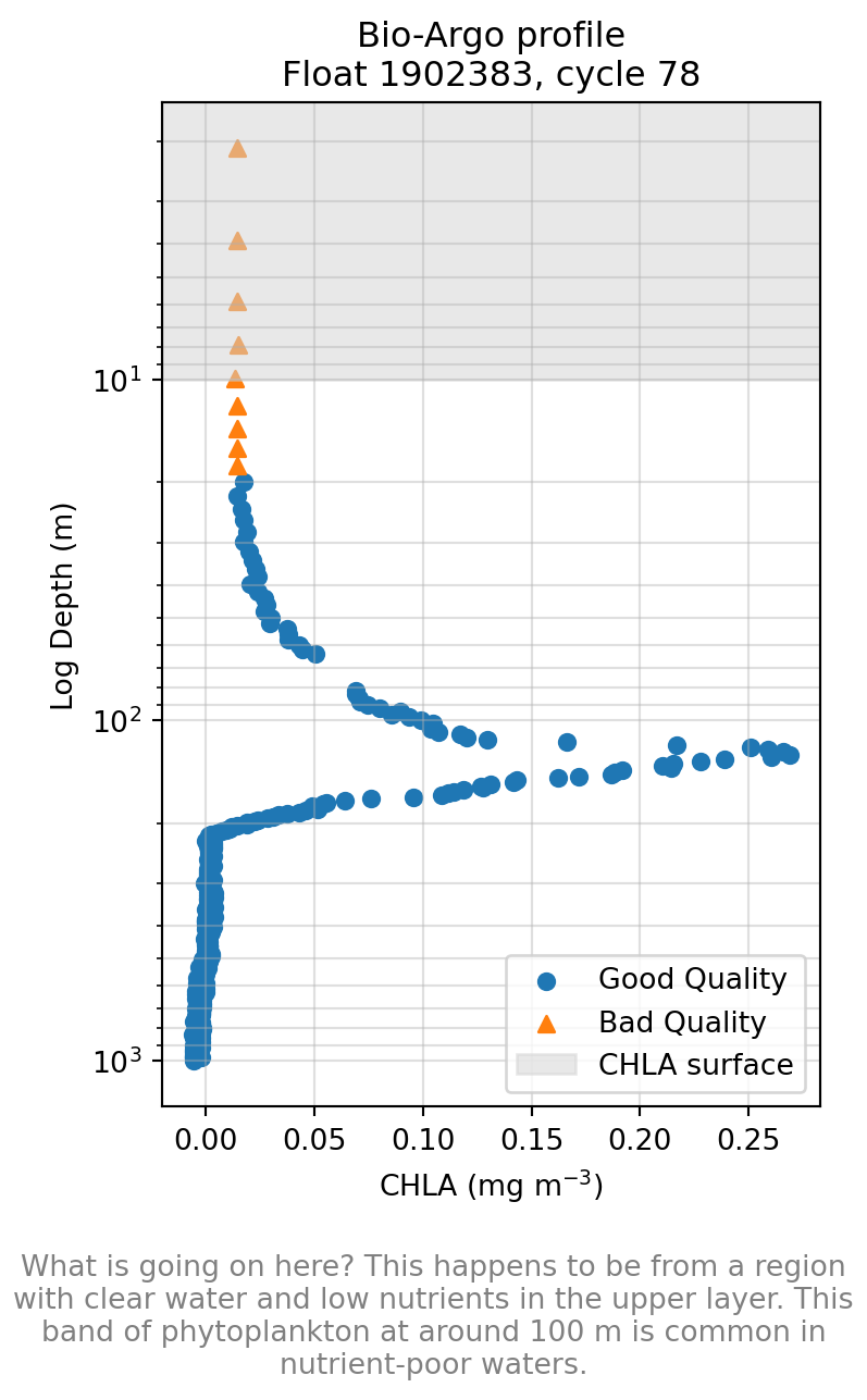
A Chlorophyll Profile from an BGC-Argo Buoy
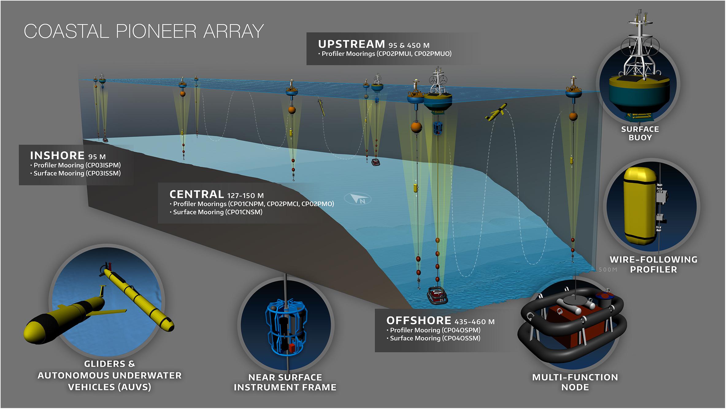
Ocean Observing Initiative (OOI)
- Fixed moorings with fluorometers at discrete depths
- High-frequency CHLA, temperature, salinity
- Key for shallow structure, seasonal cycles, and diel variability
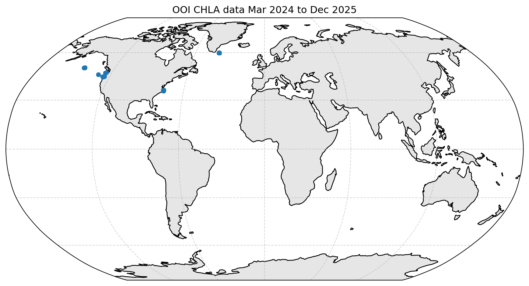
OOI Provides Coastal and Shelf Data
Performance
Overall we see a close match between our predictions and our test data for CHLA in the upper 10m — for non-coastal data.
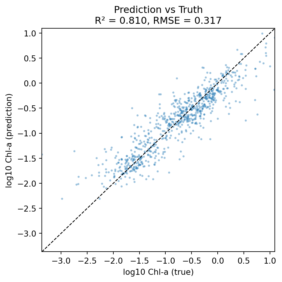
Prediction of CHLA 0 to 10m
Using PACE data for hyperspectral Rrs, we can make a prediction of surface CHLA. Let’s compare to PACE’s surface CHLA product as a first pass check, but note that these are different products trained on different in-situ data. Note surface CHLA is not our goal.
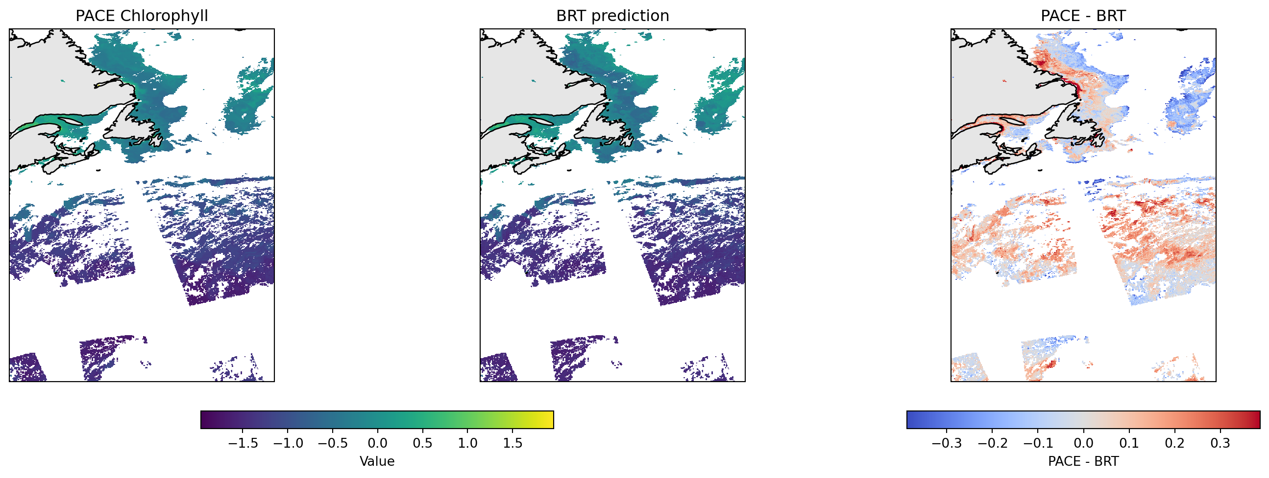
We do not expect these to be identical as the PACE chlor_a is based on the classic Rrs ratio algorithm while the BRT uses the whole spectrum but most importantly was trained on Argo and OOI florometer measurements.
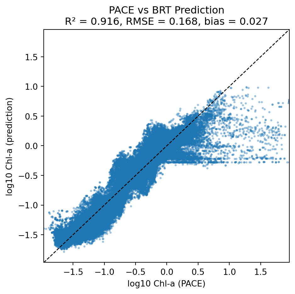
Scatter plot
PACE chlor_a to BRT with type = 1 (ooi) and solar_hour = 0 (midnight)
Notice that at high PACE chlor_a, the BRT model predicts lower CHLA_0_10. We might be able to correct this by using the whole CHLA depth profile (next section).
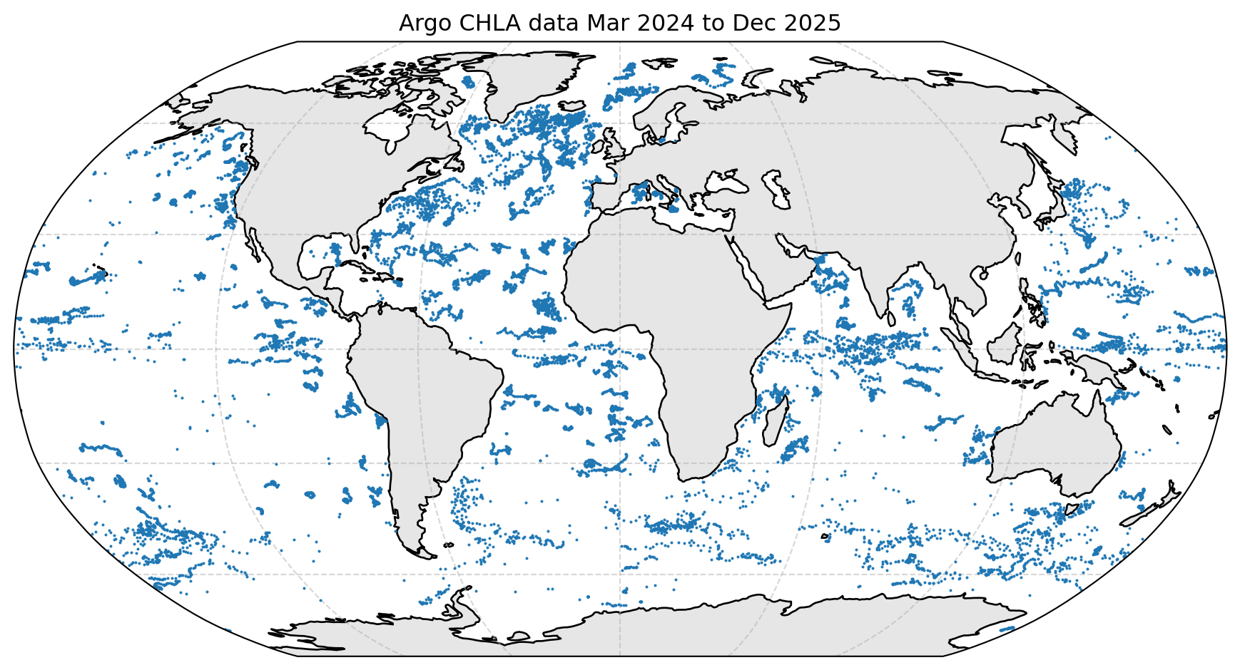
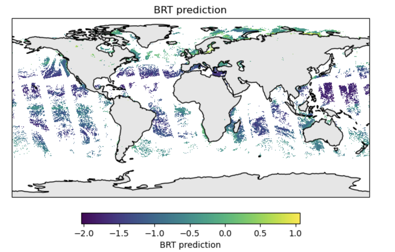
Global prediction
We can do this for the whole globe.
CHLA Profiles: Observed vs BRT
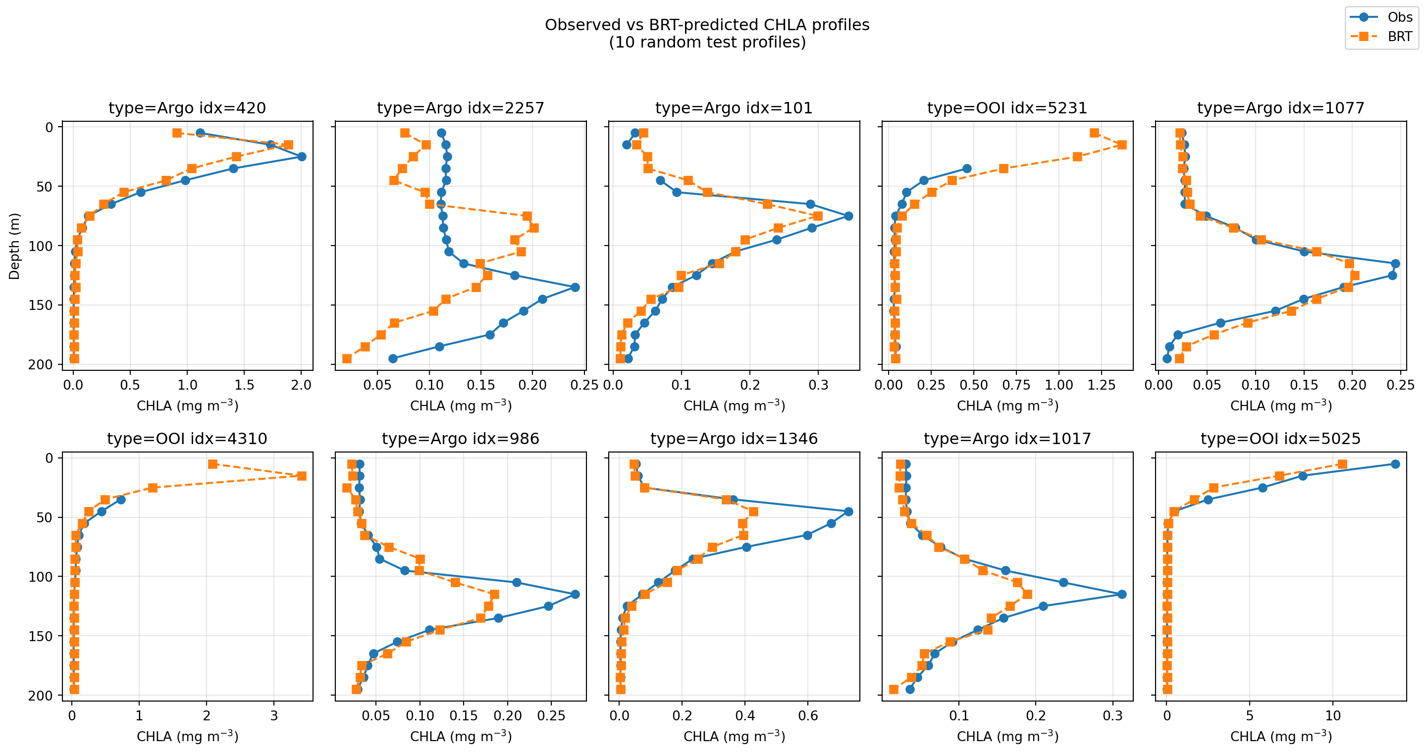
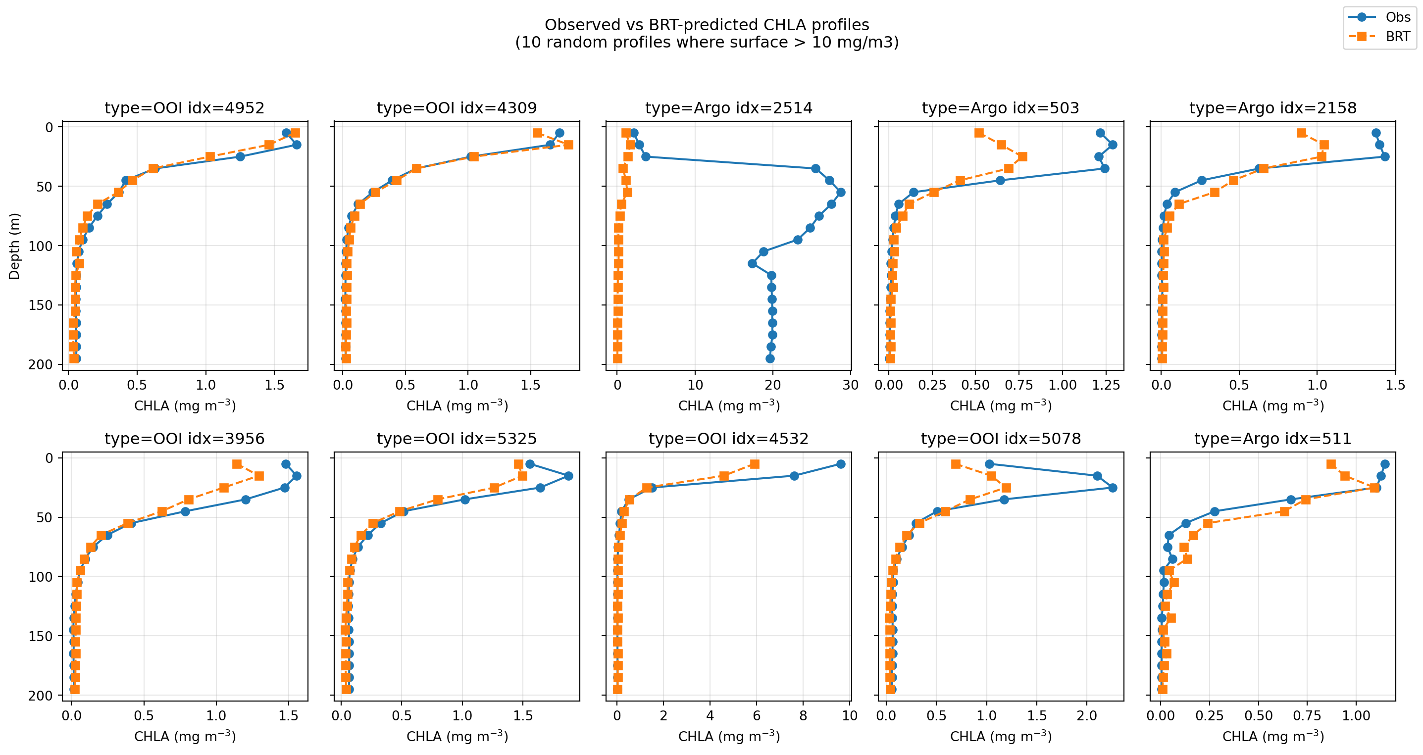
When surface CHLA is high?
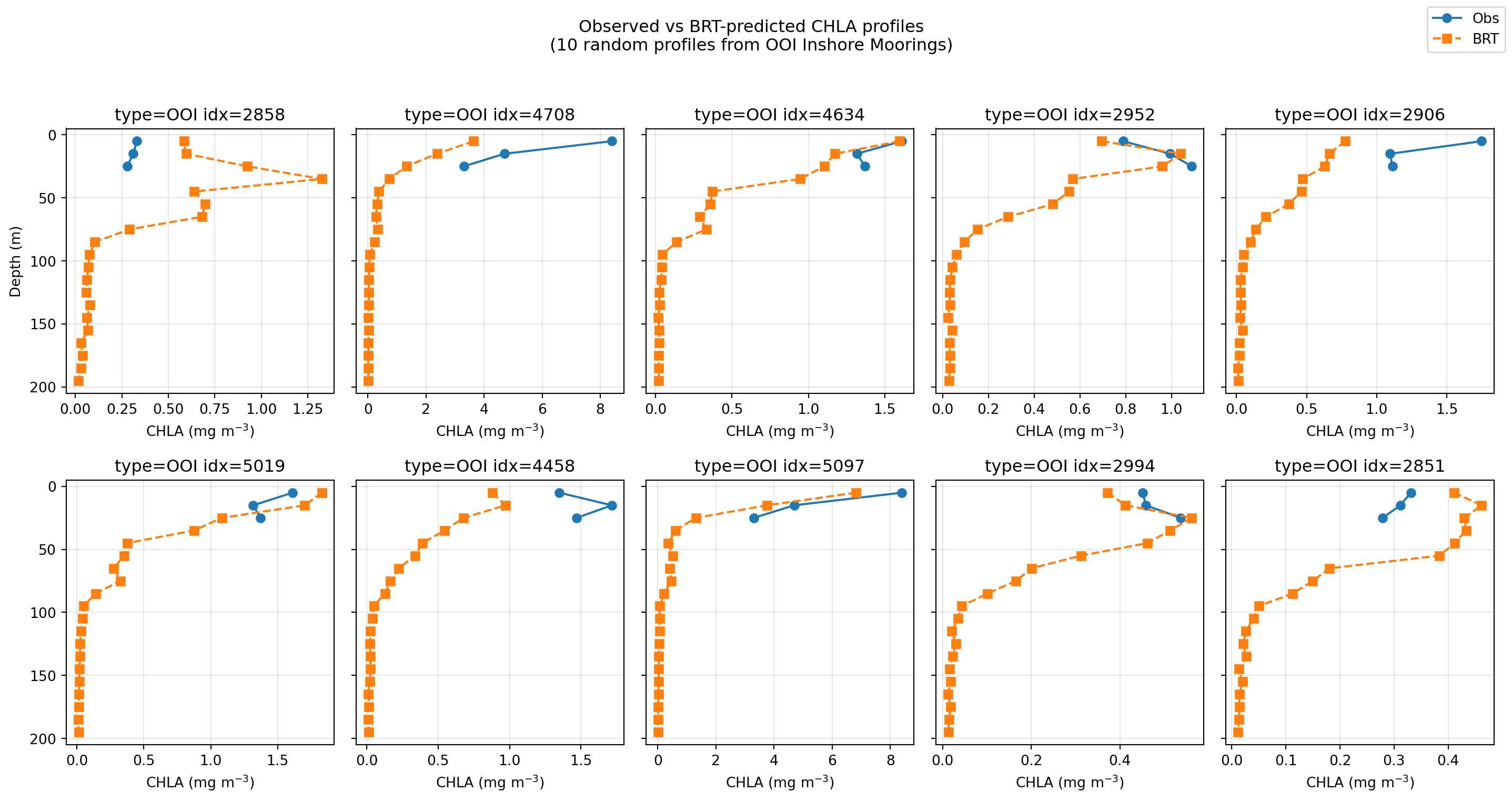
Coastal waters?
Not enough data yet. No correction was done for bathymetry (scattering off bottom), so that will need to be fixed for shallow water.
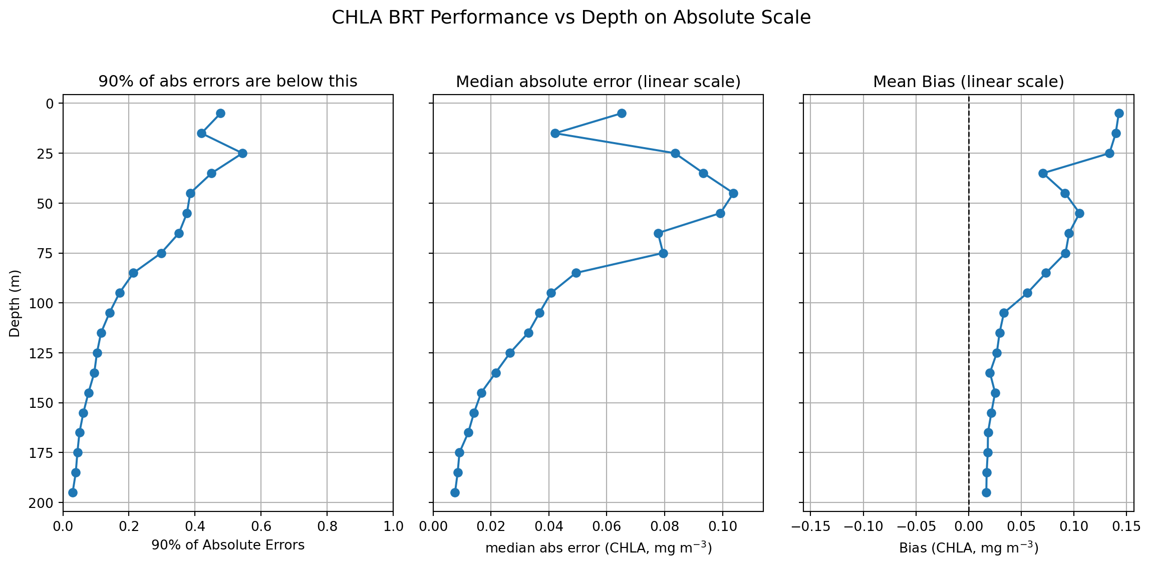
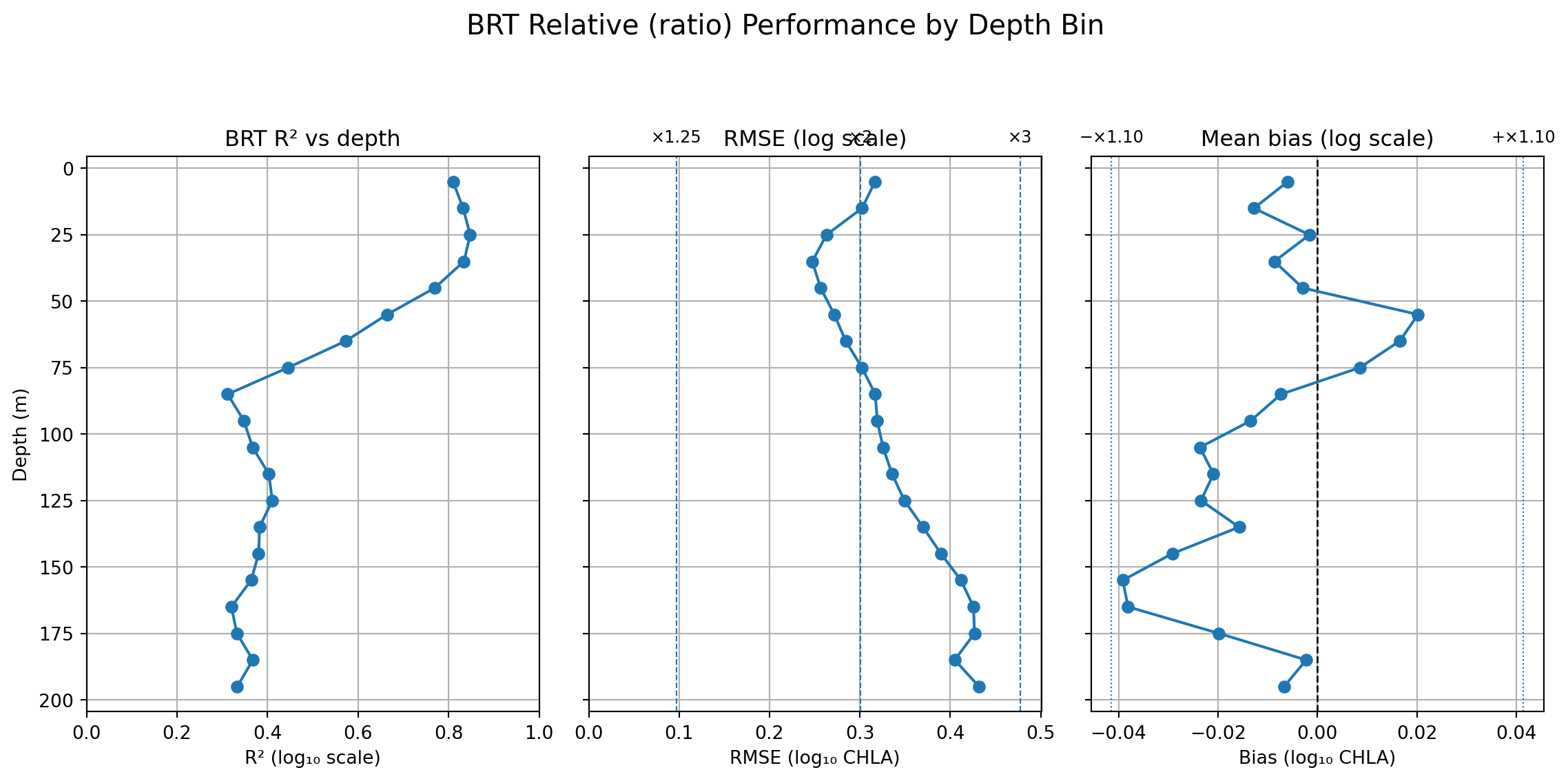
Absolute Errors for Depth Bins
Proportional Errors for Depth Bins
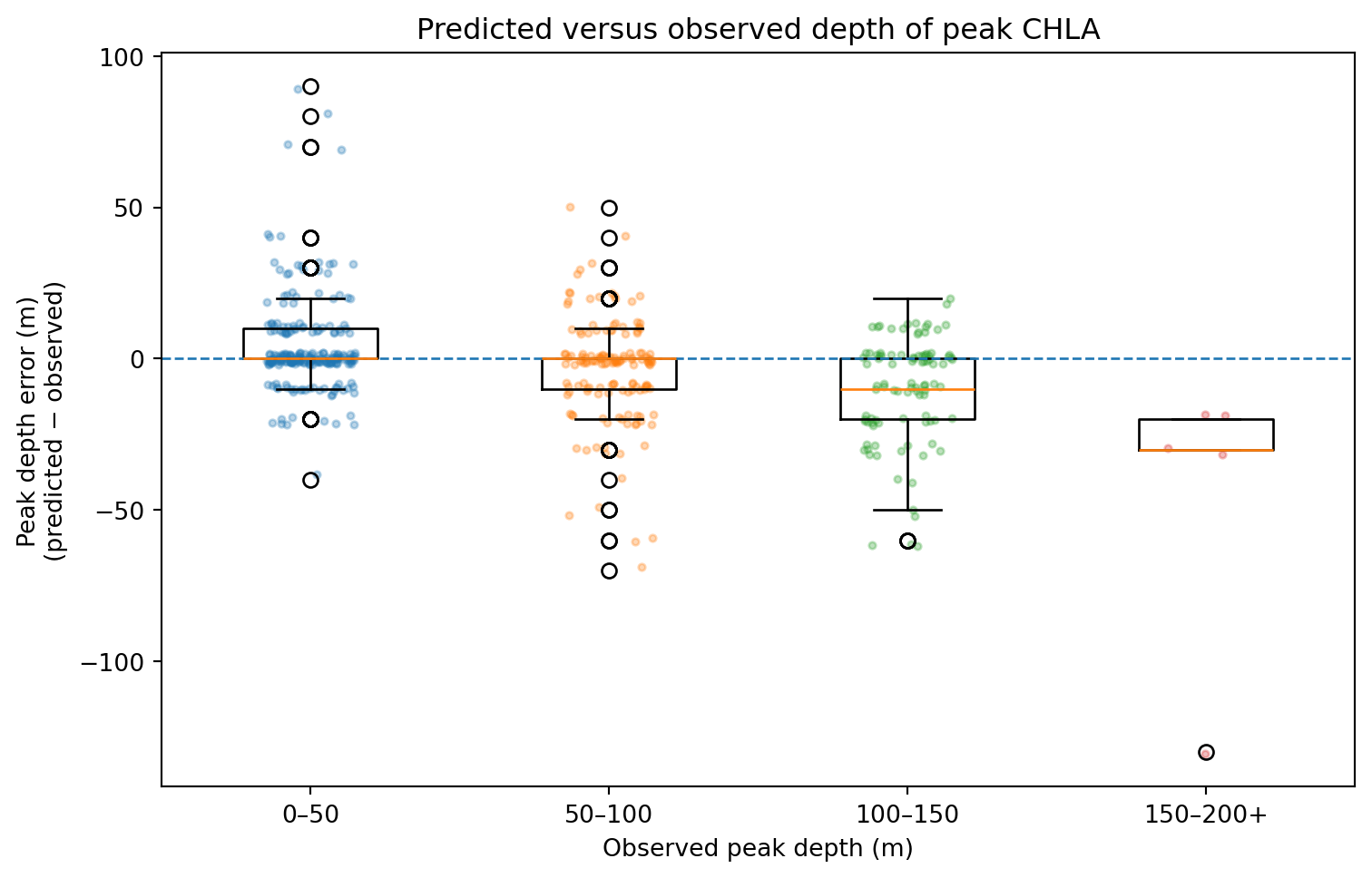
Peak Depth and Height
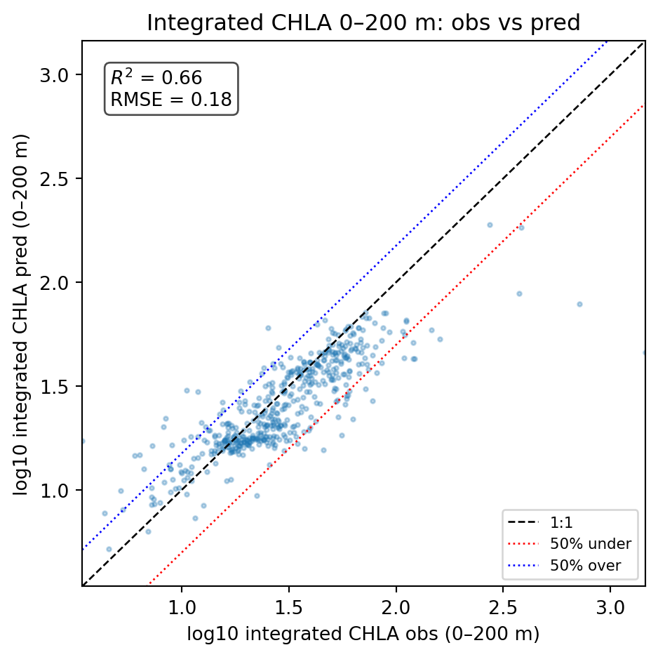
Integrated CHLA (0–200 m)